66 One-Way ANOVA

Test Review

A: Test hypothesis:

Null Hypothesis (H₀): µ₁ = µ₂ = µ₃  = …   = µ_k  (The difference of population means among all independent groups are equal)

Alternative Hypothesis (Ha): at least one group mean is not equal (At least one of the group population means is not equal to others)

where µ₁ to µ_k represent the population mean of the groups involved in one study (k>=3). The One-way ANOVA is an omnibus test meaning the test results can only tell you the overall difference among groups. If researchers are interested in the differences between any of the subgroups, follow-up comparison tests are required.

B: Test Statistic:

We consider different sources of variance to calculate the test statistics F.

between-group variance: variation due to differences between group means.

within-group variance: variation within the involved groups, also called error.

F=MSBMSW

Where

SST = the total sum of squares – which is the sum of SSB and SSR.

SSB= the sum of squares for between- group.

SSW = the sum of squares for within group (error).

Then there are corresponding degrees of freedom for all three terms.

df_T = the total degrees of freedom (df_T = n – 1)

df_B = the between-group degrees of freedom (equal to df_B = k – 1)

df_w = the within-group degrees of freedom (equal to df_W = n – k)

k = the total number of independent groups

n = the sample size

MSB = SSB/df_B = the mean square between-group

MSW = SSW/df_W = the mean square within-group (error)

C: Statistical decision

If the p-value is less than α (commonly defined as 0.05), you reject the null hypothesis and conclude that there is a significant difference in the means across all the groups.
If the p-value is greater than α, you fail to reject the null hypothesis and conclude that there is not enough evidence to suggest a significant difference among the group means.

Sample scenario:

In an educational study, researchers are investigating the effect of television commercials on the attention spans of 9-year-old children. The study measures how long the children can maintain focus during commercials for different product categories, including clothes, food, and toys. Children are randomly assigned to one of the three groups. The attention span of each child is recorded to determine if there are differences when children review different types of commercials.

Procedures:

Step A: Develop the test hypothesis.

Ho: The mean attention span of 9-year-old children is the same across all three groups (clothes, food, and toys).

Ha: At least one of the group means is different.

Step B: Perform the one-Way ANOVA.

Open the data file named OnewayANOVA.sav in SPSS.

Data Set-up: Your data should include two variables. One is the grouping variable with three or more categories. The other variable is continuous.

Running the test:

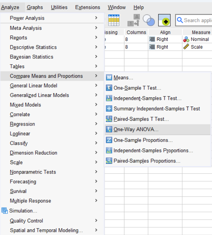
Click Analyze > Compare Means and Proportions > One-Way ANOVA.

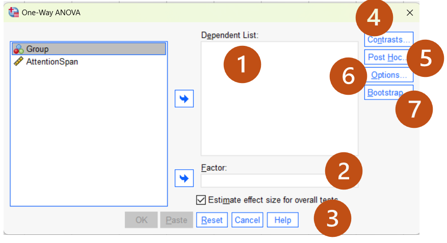
• Dependent list: The variable of the mean comparison (e.g., AttentionSpan).
• Factor: The grouping variable defining all the compared groups. In ANOVA, we have three or more categories (e.g., Group).
• Estimate effect sizes for overall tests: Generate the effect size estimates. You may un-select that option for now.
• Contrasts (optional): Specify contrasts, or planned comparisons, for subgroups after the overall ANOVA test. Click the button for more detailed information. Keep the default options for now.
• Post Hoc (optional): Request post hoc (also known as multiple comparisons) tests. Click the button for more detailed information. Specific post hoc tests can be selected by checking the associated boxes. Keep the default options for now.
• Options: Clicking “Options” opens a window where you can ask for additional output. We will not introduce the detailed information in the tutorial. We will ask for additional descriptive information when we run the test (see below).
• Bootstrap: Click “Bootstrap” to check the stability of the testing results. We will not cover this feature in the course.

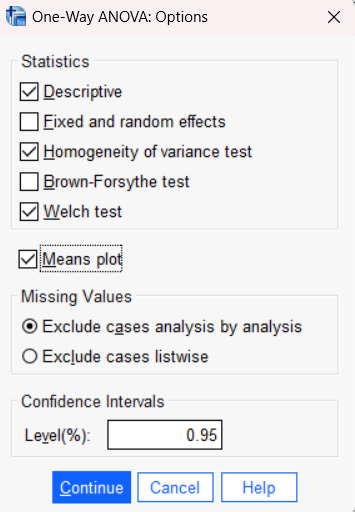
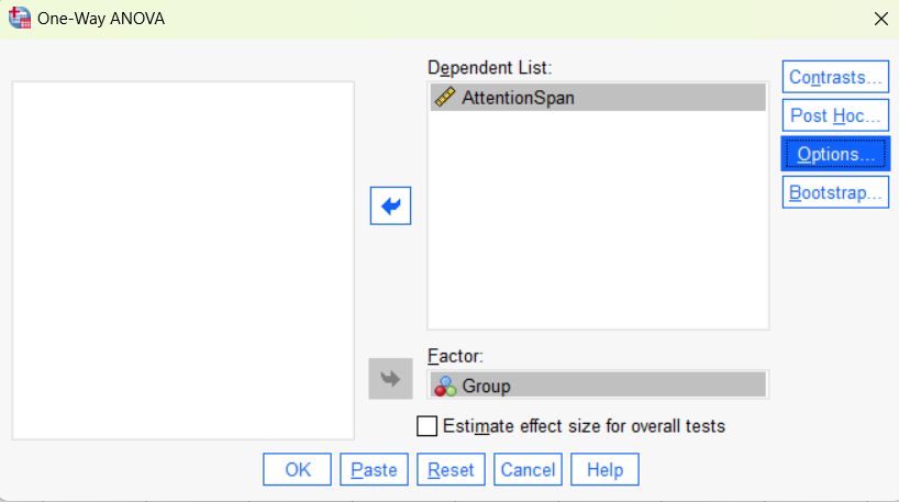
Move the variable “AttentionSpan” to “Dependent List”, “Group” to “Factor” and un-check “Estimate effect sizes for overall tests.” Next, click “Options.” Check “Descriptive” and “Means plot.” This will help us generate descriptive statistics for the results interpretation. We will also check the “Homogeneity of variance test” and “Welch test.” As in the independent t test, we need to examine the homogeneity of variance among groups using Levene’s test. If the assumption is violated (i.e., p <.05), we need to explain the results of the “Welch test” instead of the original ANOVA F-test result. Keep other options as default.

Click Continue to return to the previous testing window. After you set up the test as shown in the table below, click OK to run the test.

 

Output (4 tables and 1 figure):

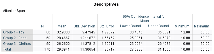
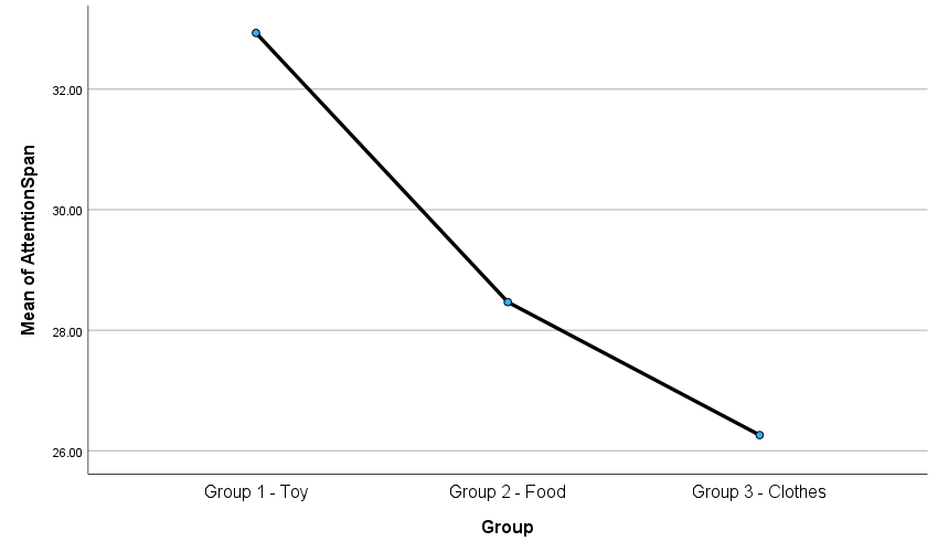
Interpreting the descriptive statistics is a preliminary step before analyzing the inferential results. SPSS initially provides descriptive statistics for each group, including the mean, N, standard deviation, standard error of the mean, 95% confidence interval for the mean, as well as the minimum and maximum values. The results show that the group exposed to toy commercials had a longer attention span compared to the other two groups (i.e., food or clothes), with lower score variability. A similar pattern can be observed in the mean plot below.

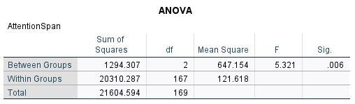
This is the key output table – ANOVA. We can identify the Sum of square values and the Mean of Square Values as illustrated in the ANOVA formula.

SST = 21604.594 (df_T = 169)

SSB= 1294.307 (df_B = 2)

SSW = 20310.287 (df_w =167)

MSB = SSB/df_B = 647.154

MSW = SSW/df_W = 121.618

F (2,167) = MSB/MSW= 5.32 (p=.006)

Before we interpret the original ANOVA results, let’s examine the homogeneity test results first.

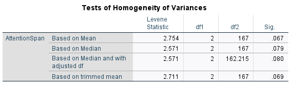
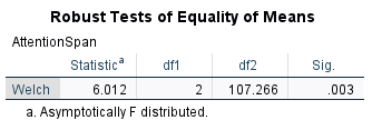
There was homogeneity of variances, as assessed by Levene’s test for equality of variances (p = .067). Therefore, we can rely on the original ANOVA result. If the p-value of the homogeneity test is below .05, we would need to interpret the result of the “Robust Test of Equity of Means.”

Step C: Results Interpretation

Based on the p-value, we reject the null hypothesis that the mean difference in the attention span seconds among the three groups is zero. We conclude that the mean attention span seconds is significantly different for at least one of the commercial groups, F (2,167) = 6.35, p = .002.

As ANOVA does not tell us which means were different from one other, we need to follow up with the post-hoc tests. You may review the relevant content in SPSS explained.

Measures of Associations