63 Chapter 2: Foundations
Chapter Overview
Before we discuss the statistical tests covered, we will briefly review the basic statistics and relevant concepts that will benefit our learning of more advanced statistical tests. We will employ the open resource database from the High School Longitudinal Study of 2009 to demonstrate the statistical procedures (https://nces.ed.gov/surveys/hsls09/).
2.1 Descriptive Statistics
Research methods texts and research articles clearly state descriptive statistics are the essential first step in data analysis, as they summarize and reveal patterns in the data; while inferential statistics techniques allow us to conduct tests on samples and generalize results to the population from which they were from (Gravetter & Wallnau, 2017; Keselman et al., 1998). In order to summarize the data, it is essential to learn different measurement scales.
Categorical variables (nominal or ordinal): The variables can be grouped into distinct categories. Examples include gender, race, or academic rank. Nominal variables have categories without a natural order (e.g., gender), while ordinal variables have categories with a meaningful sequence (e.g., academic rank).
Numerical variables: Such variables measure quantities expressed as numbers. Examples include test scores, age, and height. Numerical variables can be converted into categories (e.g., age ranges). However, categorical variables cannot be transformed into numerical variables without losing their original meaning.
Frequency Distribution
For categorical variables, we normally report frequency table/distribution, which displays how often each value occurs in a variable (applicable to nominal scales such as gender, ordinal scales such as agreement levels in an item).
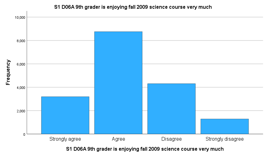
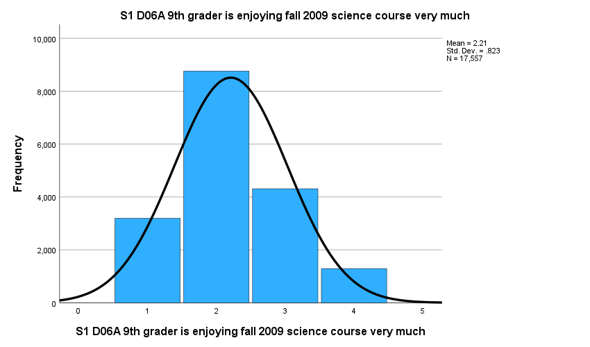
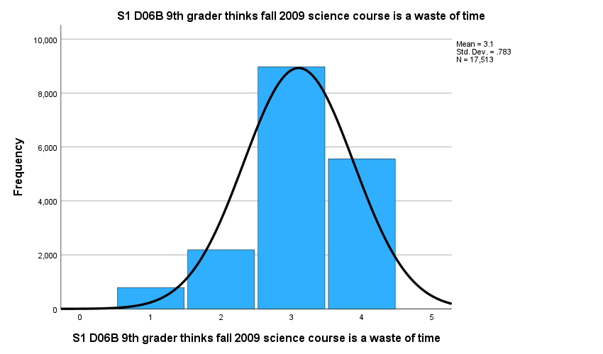
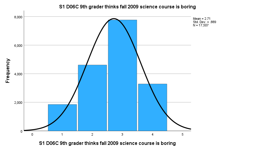
Example: We intend compute frequencies of three variables that measure science interest levels of 9th-grade students (S1SENJOYING, S1SWASTE, S1SBORING).
S1SENJOYING = 9th grader is enjoying fall 2009 science course very much (label)
S1SWASTE = 9th grader thinks fall 2009 science course is a waste of time (label)
S1SBORING = 9th grader thinks fall 2009 science course is boring (label)
Tips: Please check if all the items are worded in the same direction. Consider how this may influence data analysis.
SPSS Procedure:
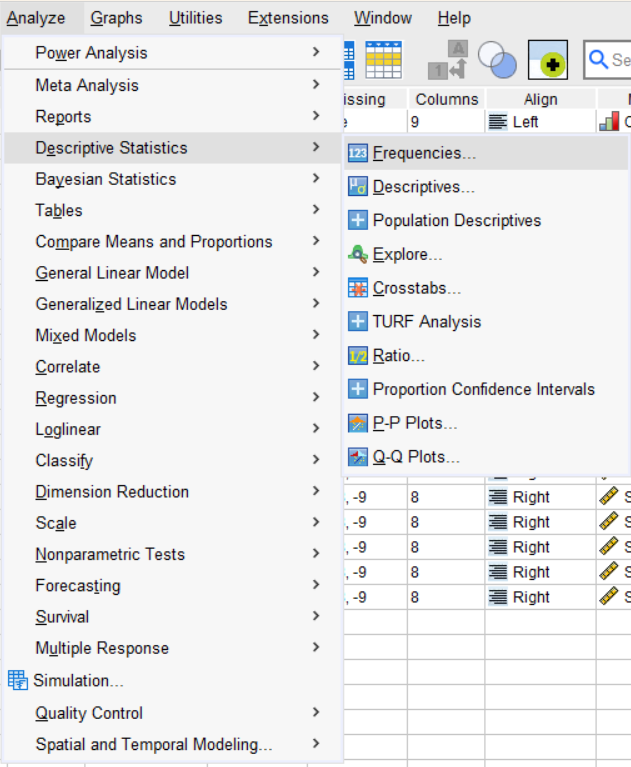
- Select Analyze > Descriptive Statistics > Frequencies.

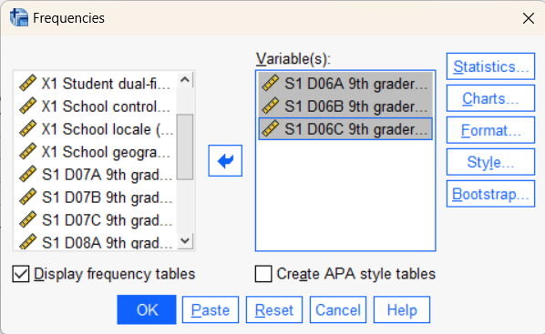
- From the window of “Frequencies,” select the variables of interest. Check the box “Display frequency tables.”

We can right-click on the mouse to change the setting of displaying variables. Let’s select “Display Variable Labels” (default setting) so the results are easier to follow.

- In addition to the frequency table, we can obtain charts related to the frequency of a variable. Select Chart. We can select the chart after the window pops up. Let’s select Bar Charts as an example.
- Select Continue to return to the window of Frequencies and then select OK to generate the output.
Output (selected):
|
S1 D06A 9th grader is enjoying fall 2009 science course very much |
|||||
|
|
Frequency |
Percent |
Valid Percent |
Cumulative Percent |
|
|
Valid |
Strongly agree |
3194 |
13.6 |
18.2 |
18.2 |
|
Agree |
8762 |
37.3 |
49.9 |
68.1 |
|
|
Disagree |
4310 |
18.3 |
24.5 |
92.6 |
|
|
Strongly disagree |
1291 |
5.5 |
7.4 |
100.0 |
|
|
Total |
17557 |
74.7 |
100.0 |
|
|
|
Missing |
Missing |
277 |
1.2 |
|
|
|
Unit non-response |
2059 |
8.8 |
|
|
|
|
Item legitimate skip/NA |
3610 |
15.4 |
|
|
|
|
Total |
5946 |
25.3 |
|
|
|
|
Total |
23503 |
100.0 |
|
|
|
Note: The variable label (i.e., S1 C06A 9th grader is enjoying fall 2009 science course very much) is displayed as the table title.
Central Tendency and Variability
While we can compute frequency distributions to numerical variables (e.g., scores from a test or a survey scale), we are normally more interested in learning the data features by asking these questions:
- What is the central tendency of a variable?
Median – midpoint of a distribution; 50th percentile
Mean – Sum of scores divided by a total number of scores.
- What is the variability of a variable?
- Range: The difference between the highest and lowest scores
- Deviation score: the difference between a single score and the mean score of a variable
- Variance: the mean of the squared deviation scores
- Standard Deviation: the square root of the variance (the amount of variation for the scores from its mean)
SD=(X-Mean)2N
- What is the shape of the distribution?
- Symmetry or not: Skewness (symmetric if the left and right sides of the distribution look the same)
- Tails of the distribution: Kurtosis (if the variable has values mostly around the mean or to the tails of the distribution)
- The values for skewness and kurtosis between -2 and +2 are considered acceptable to follow distribution (George & Mallery, 2010).
- The shape of the distribution can be visualized using histogram.
Tips: Mean and standard deviation are typically reported in research articles.
Example: We can consider three variables related to science interest (S1SENJOYING, S1SWASTE, S1SBORING) and compute the descriptive statistics. We will introduce two ways to obtain descriptive statistics.
SPSS Procedures (Option 1):
- Select Analyze > Descriptive Statistics > Descriptives.
- Select the variables of interest after the Descriptives window pops up.
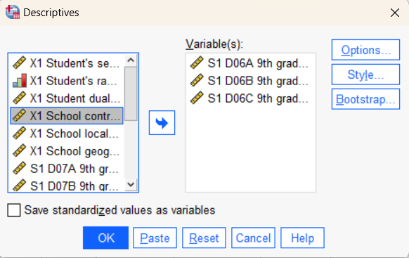
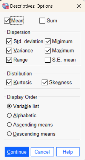
- After selecting the variable of interest, select Options to check descriptive statistics boxes: Mean, Standard Deviation, Variance, Minimum, Maximum, Range, Kurtosis, and Skewness.
- Select Continue to return to the window of Descriptives and then select OK to generate the output.
Output:
|
Descriptive Statistics |
|||||||||||
|
|
N |
Range |
Minimum |
Maximum |
Mean |
Std. Deviation |
Variance |
Skewness |
Kurtosis |
||
|
Statistic |
Statistic |
Statistic |
Statistic |
Statistic |
Statistic |
Statistic |
Statistic |
Std. Error |
Statistic |
Std. Error |
|
|
S1 D06A 9th grader is enjoying fall 2009 science course very much |
17557 |
3 |
1 |
4 |
2.21 |
.823 |
.677 |
.385 |
.018 |
-.294 |
.037 |
|
S1 D06B 9th grader thinks fall 2009 science course is a waste of time |
17513 |
3 |
1 |
4 |
3.10 |
.783 |
.613 |
-.746 |
.019 |
.392 |
.037 |
|
S1 D06C 9th grader thinks fall 2009 science course is boring |
17507 |
3 |
1 |
4 |
2.71 |
.889 |
.791 |
-.307 |
.019 |
-.610 |
.037 |
|
Valid N (listwise) |
17443 |
|
|
|
|
|
|
|
|
|
|
SPSS Procedure (Option 2)
The frequency procedure can provide similar descriptive statistics.
- Select Analyze > Descriptive Statistics > Frequencies.
- From the window of “Frequencies,” select the variables of interest. Uncheck the box “Display frequency tables” if you are interested in obtaining the descriptive statistics only.
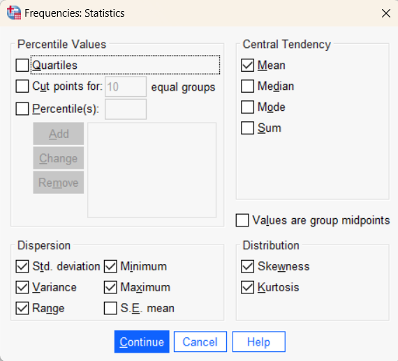
- After selecting the variables of interest, select “Statistics” to check the descriptive statistics boxes: Mean, Standard Deviation, Variance, Minimum, Maximum, Range, Kurtosis, and Skewness.
- Select Continue to return to the window of Frequencies and select Chart to obtain a histogram of selected variables.
- Select Continue to return to the window of Frequencies and OK to generate the output.
Output
|
Statistics |
||||
|
|
S1 D06A 9th grader is enjoying fall 2009 science course very much |
S1 D06B 9th grader thinks fall 2009 science course is a waste of time |
S1 D06C 9th grader thinks fall 2009 science course is boring |
|
|
N |
Valid |
17557 |
17513 |
17507 |
|
Missing |
5946 |
5990 |
5996 |
|
|
Mean |
2.21 |
3.10 |
2.71 |
|
|
Std. Deviation |
.823 |
.783 |
.889 |
|
|
Variance |
.677 |
.613 |
.791 |
|
|
Skewness |
.385 |
-.746 |
-.307 |
|
|
Std. Error of Skewness |
.018 |
.019 |
.019 |
|
|
Kurtosis |
-.294 |
.392 |
-.610 |
|
|
Std. Error of Kurtosis |
.037 |
.037 |
.037 |
|
|
Range |
3 |
3 |
3 |
|
|
Minimum |
1 |
1 |
1 |
|
|
Maximum |
4 |
4 |
4 |
|
Note: The same descriptive statistics are obtained with different layout styles using two options.
Based on descriptive statistics, we can assume all variables are normally distributed based on skewness and kurtosis values. The mean values of the three items are different, indicating varied agreement levels of these items. The standard deviations (variability) of the three items are similar across variables. The figures below provide similar information.
2.2 T tests and ANOVA
We will review how to compute the following statistical tests in this section.
- One-sample t-test.
- Paired t-test.
- Independent t-test.
- One-way ANOVA.
Data files used to run the analysis will be provided by the instructor with the corresponding test names. Each test includes the following elements: a brief test review including test hypothesis, test statistics, and statistical decision; a research scenario for the corresponding test, and procedures with these elements: developing test hypothesis, performing the test in SPSS, and interpreting statistical results.
One-sample t test
Test Review
A: Test hypothesis:
Null Hypothesis (H₀): µ = µ0 (The mean is equal to a specific mean value)
Alternative Hypothesis (Ha): µ ≠ µ0 (The mean is NOT equal to a specific mean value; we can change it to a one-sided test)
B: Test Statistic:
t=x̅-μ0sn
Where:
x-bar is the sample mean;
is the hypothesized population mean;
s is the sample standard deviation;
n is the sample size.
The degrees of freedom (df) is n-1. This is used to identify the critical t-value from the t-distribution to make the statistical decision.
C: Statistical decision
If the p-value is less than α (commonly defined as 0.05), you reject the null hypothesis , concluding that there is a significant difference between the population mean and the hypothesized mean.
If the p-value is greater than α, you fail to reject the null hypothesis, concluding that there is not enough evidence to suggest a significant difference.
Sample scenario
The national average SAT score is 890. The Superintendent of New York City schools wants to determine if the average SAT score of students in the city’s schools is significantly lower than the national average. Conduct a statistical test to evaluate this question and make a decision.
Procedures
Step A: Develop the test hypothesis.
Ho: µ = 890.
Ha: µ < 890.
Step B: Perform the one-sample t test
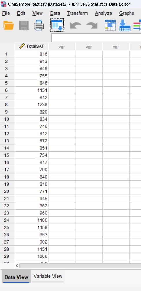
Open the data file named One-sampleTtest. sav in SPSS. Select File > Open > Data (open *.sav file); Select One-sampleTtest.sav > Open. (Note: As the process is similar to other tests, we will not repeat this step again).
Data Set-up: The data should include one continuous variable (e.g., test scores).
Running the test:
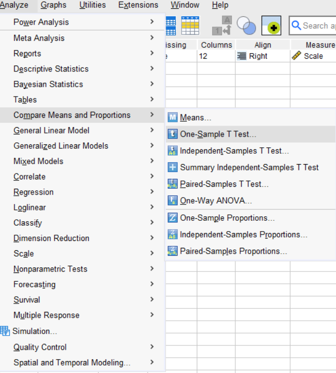
Click Analyze > Compare Means and Proportions > One-Sample T Test.
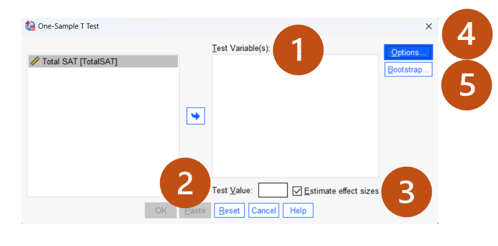
Test Window Review:
- Test Variable(s): Select the test variable (e.g., TotalSAT) to be compared to the hypothesized population mean (i.e., Test Value in #2).
- Test Value: Enter the hypothesized population mean (e.g., 890).
- Estimated Effect Sizes: Generate the effect size estimate. You may leave the option unselected option for now.
A quick introduction to the statistical and practical significance.
Statistical significance indicates whether an observed effect or relationship in the data is unlikely to have occurred by chance. It is determined through inferential statistical tests, such as t-tests, or ANOVA, which provide p-values to assess the likelihood that the results are due to chance.
Practical significance assesses whether that effect or relationship is meaningful in practice, regardless of statistical significance. It is measured by effect size, which quantifies the strength or magnitude of the observed relationship or difference. Different effect size indices are associated with different inferential statistical tests. You may review more information on effect size from this book.
Options: Click “Options” to adjust the confidence interval percentage and handle missing data. Keep the default settings.
- Bootstrap: Click “Bootstrap” to check the stability of the testing results. We will not cover this feature in the course. If you purchase the SPSS Explained, you can find more detailed interpretations in Chapter 6.
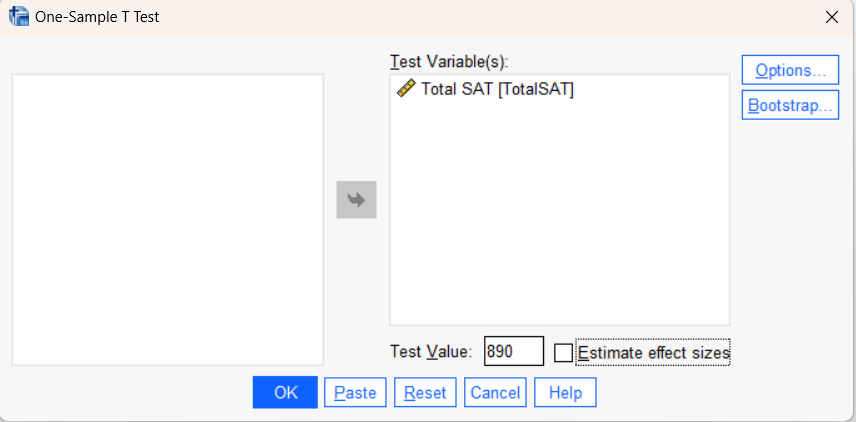
Move The test variable “TotalSAT” to Test Variable(s), enter 890 as the Test Value, and un-check “Estimate effect sizes.” After you set up the test as shown in the table below, click “Okay” to run the test.
Output (two tables):
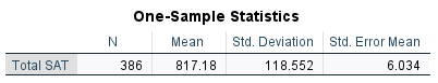
Remember that it is essential to interpret the descriptive statistical results as a preliminary step before analyzing the inferential statistics. The descriptive results show that the mean SAT score is 817.18, which is lower than the national average of 890.
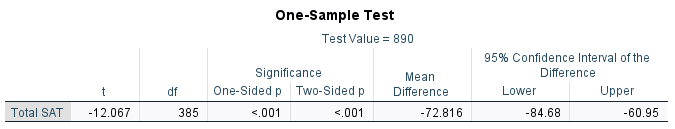
This is the key output table – One-Sample Test.
Test Value: The hypothesized value entered in the testing window with a value of 890.
t: The test statistic for the one-sample t test with a value of -12.07.
df: The degrees of freedom for the test with a value of 385.
Significance (one-sided p and two-sided p): The p-values associated with the t test. The conclusion is the same no matter if you conduct a one or two-sided test in this example.
Mean difference: The mean difference between the sample mean and the hypothesized population mean.
95% Confidence Interval for the Difference: The confidence interval for the true mean difference. We are 95% confident that the mean difference between the New York SAT average and the National SAT average is between -84.68 and -60.95.
Step C: Results Interpretation
Based on the p-value above, we reject the null hypothesis that the mean SAT score in New York schools is equal to the population mean of 890. The results indicate that the mean SAT score in New York schools (M = 817.18, SD = 118.55) is significantly lower than the population mean, t (385) = -12.07, p < .001.
