65 Independent t test

Test Review

A: Test hypothesis:

Null Hypothesis (H₀): µ₁ = µ₂ (The difference of population means between two independent groups are equal)

Alternative Hypothesis (Ha) µ₁ ≠ µ₂ (The difference of population means between two independent groups is not equal)

where µ₁ is the population mean of group 1, and µ₂ is the population mean of group 2. It was noted that the hypothesis looks similar compared to the Paired t test. The difference is that we have two independent groups in the independent t test. We can specify a one-sided Ha based on the research scenario.

B: Test Statistic:

t=x1-x2sp1n1+1n2

Where:

is the sample mean of Group 1;

is the sample mean of Group 2;

is pooled standard deviation (formula not shown here);

is the sample size of Group 1;

is the sample size of Group 2;

The degrees of freedom (df) is

to identify the critical t-value from the t-distribution to make the statistical decision.

C: Statistical decision

If the p-value is less than α (commonly defined as 0.05), you reject the null hypothesis ​and conclude that there is a significant difference between the means of the two independent groups.
If the p-value is greater than α, you fail to reject the null hypothesis and conclude that there is not enough evidence to suggest a significant difference between the means of the two independent groups.

Sample scenario

A group of researchers are interested in investigating whether blind children score significantly different on the perceived motor competence scale compared to nonblind children. The perceived motor competence score is used to assess children’s competency levels. Children in the study are grouped based on their vision status (nonblind = 0, blind = 1).

Procedures

Step A: Develop the test hypothesis.

Ho: The difference in the mean competency cores between the blind and non-blind children is zero.

Ha: The difference in the mean competency scores is higher for non-blind children compared to blind children.

Step B: Perform the independent t test.

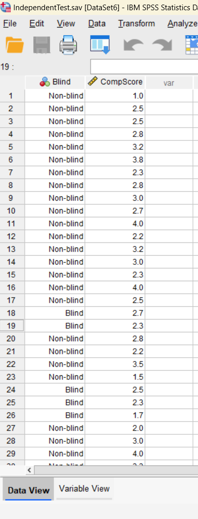
Open the data file named IndependentTtest.sav in SPSS.

Data Set-up: Your data should include two variables. One is the grouping variable with two categories (e.g., blind or non-blind). The other variable is continuous (e.g., scores).

Running the test:

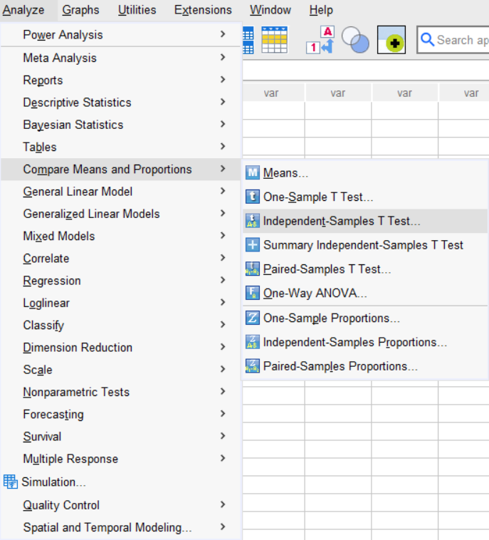
Click Analyze > Compare Means and Proportions > Independent-Samples T Test.

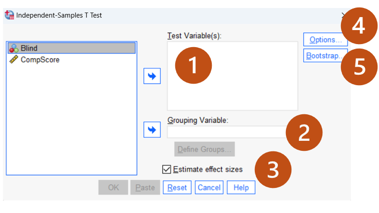
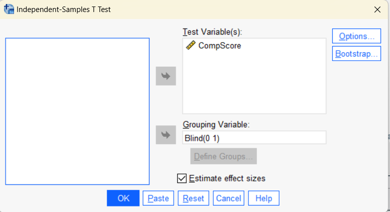
Let’s review the test window together.

• Test Variable(s): This is the continuous variable used for mean comparison between the two groups (e.g., CompScore).
• Grouping Variable: This is the grouping/categorical variable used to define the two independent groups (e.g., Blind).
• Define Groups: Click “Define Groups” to specify the category indicators for the test (0 or 1 in this example). The button is inactive since the grouping variable has not been entered. We will demonstrate how to define it below.
• Estimate Effect sizes. Generate the effect size estimate. You may un-select that option for now.
• Options: Click “Options” to adjust the confidence interval percentage and handle missing data. Keep the default settings.
• Bootstrap: Click “Bootstrap” to check the stability of the testing results. We will not cover this feature in the course. If you purchase the SPSS Explained, you can find more detailed interpretations in Chapter 6.

Move the variable “CompScore” to “Test Variable(s)” and “Blind” to “Grouping Variable” and un-check “Estimate effect sizes.”

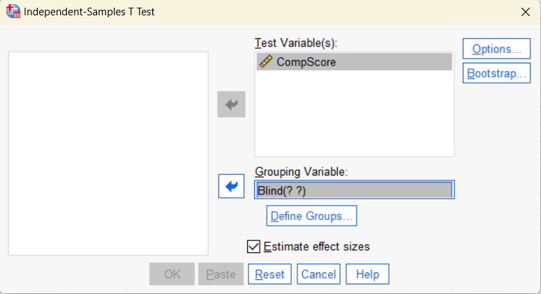
Next, click “Define Groups.” Enter 0 and 1 in Group 1 and Group 2.

 

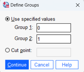
Click Continue to return to the previous testing window. After you set up the test as shown in the table below, click OK to run the test.

Output (two tables):

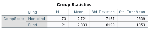
Let’s interpret the descriptive statistical results as the preliminary step before we examine the inferential statistical results. First, SPSS provides descriptive statistics for each grouping variable (mean, N, standard deviation, standard error of mean, and 95% confidence interval of the difference). The results indicate that non-blind children have higher competency scores than blind children. There are more non-blind children in the sample with higher score variability compared to those of blind children.

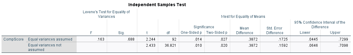
This is the key output table – Independent Samples Test.

Levene’s Test for Equity of Variances: The independent t-test requires an initial check for equality of variances between the groups, which is done using Levene’s Test for Equality of Variances. This inferential statistical test uses an F statistic. The null hypothesis states that the variances of the two groups are equal. If the p-value is less than .05, the null hypothesis is rejected, and we use the results from “Equal variances not assumed.” Conversely, if the p-value is higher than .05, we use the results from “Equal variances assumed.”

Note: The test statistics provided in the tutorial are for the “Equal variances assumed” condition. Different formulas are used for the “Equal variances not assumed” condition, which is not included in this tutorial.

In this example, we use the results from “Equal variances assumed,” as the p-value is .688.

t: the test statistics (2.24)

df: degrees of freedom (92)

Significance (One-sided p): the p-value corresponding to the given test statistic and degrees of freedom (.014). Refer to the two-sided p if needed.

Mean difference: the difference score in means between the independent groups (used to estimate the T-statistics).

Std. Error Differences:  the standard error of the mean difference estimate (used to estimate the T-statistics).

95% Confidence Interval of the Difference: The confidence interval for the mean difference. We are 95% confident that the mean difference is between .04 and .73.

Step C: Results Interpretation

Given the p-value above, we reject the null hypothesis that the mean difference in the competency scores between the two groups is zero. We conclude that the competency scores for the non-blind children (M = 2.72, SD = .72) are significantly higher than for the blind children (M = 2.33, SD = .62), t (92) = 2.24, p =.014.