64 Paired (Dependent) t test

 

Test Review

A: Test hypothesis:

Null Hypothesis (H₀): µ₁ = µ₂ (The paired means are equal)

Alternative Hypothesis (Ha) µ₁ ≠ µ₂ (The paired means are not equal; we can change it to a one-sided test)

where µ₁ is the population mean of group 1, and µ₂ is the population mean of group 2.

B: Test Statistic:

t=x1-x2sn

Where:

is the sample mean of Group 1;

is the sample mean of Group 2;

s is the sample standard deviation of the mean difference scores;

n is the sample size.

The degrees of freedom (df) is calculated as n – 1 and is used to determine the critical t-value from the t-distribution, which aids in making the statistical decision.

C: Statistical decision

If the p-value is less than α (commonly defined as 0.05), you reject the null hypothesis ​, concluding that there is a significant difference in the mean differences of the two paired groups.

If the p-value is greater than α, you fail to reject the null hypothesis, concluding that there is not enough evidence to suggest a significant difference.

Sample scenario

The pretest and posttest scores represent the mean scores on a 12-item motor skill assessment administered to children with visual impairments. Between the two assessments, the children participated in an 8-week intervention program aimed at improving their motor skills. The researcher is interested to know if the program is effective in improving these children’s motor skills.

Procedures

Step A: Develop the test hypothesis.

Ho: The mean difference between the post and pre-test scores is zero.

Ha: The mean difference between the post and pre-test scores is higher than zero.

Step B: Perform the paired t test.

Open the data file named PairedTtest. sav in SPSS.

Data Set-up: Your data should include two continuous variables (e.g., test scores) measured at two different time points or for two related conditions or units.

Running the test:

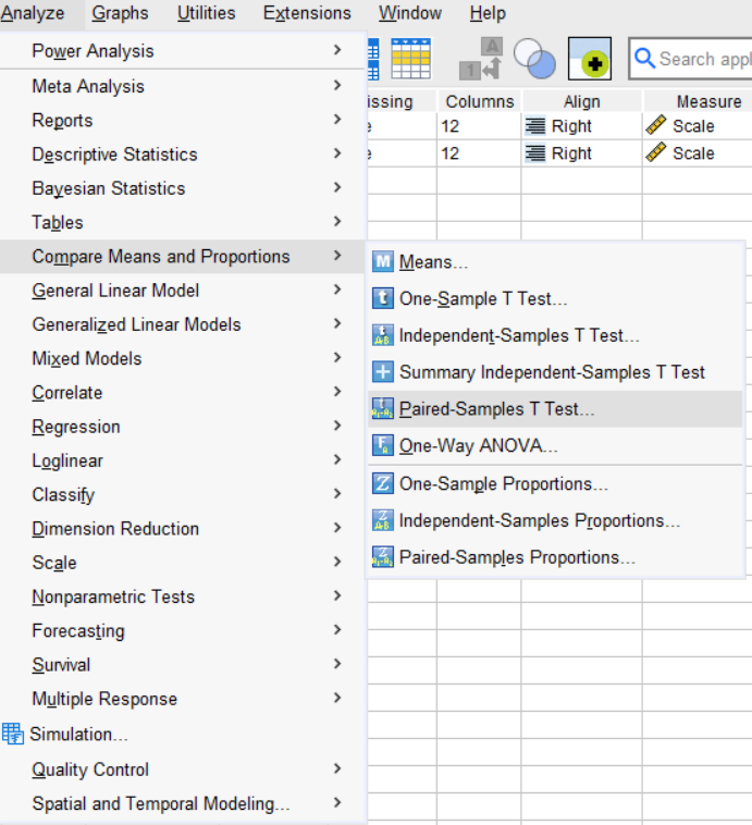
Click Analyze > Compare Means and Proportions > Paired-Samples T Test.

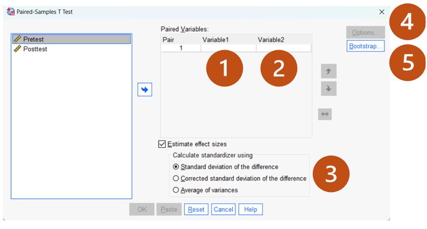
Let’s review the test window together.

1/2. The “Pair” column represents the number of paired t Tests to run. We can run multiple tests if needed. Variable 1 represents the first grouping variable and Variable 2 represents the second grouping variable identified in the test hypotheses (e.g., Variable1: Posttest; Variable 2: Pretest).

3. Estimate Effect sizes. Generate the effect size estimate. You may un-select that option for now.

4. Options: Click “Options” to adjust the confidence interval percentage and handle missing data. Keep the default settings.

5. Bootstrap: Click “Bootstrap” to check the stability of the testing results. We will not cover this feature in the course. If you purchase the SPSS Explained, you can find more detailed interpretations in Chapter 6.

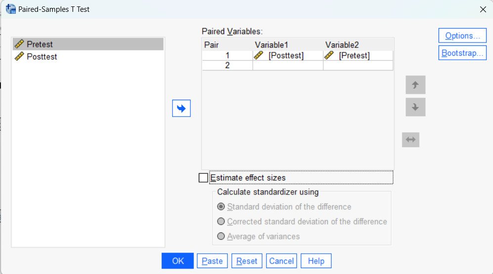
Move the variable “Posttest” to “Variable1” and “Pretest” to “Variable2” and un-check “Estimate effect sizes.” After you set up the test as shown in the table below, click “OK” to run the test.

Output (three tables):

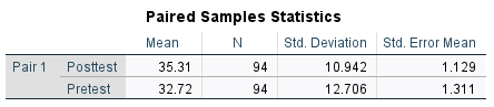
Keep in mind that interpreting descriptive statistics is a preliminary step before analyzing the inferential statistics. First, SPSS provides descriptive statistics for each grouping variable, including the mean, N, standard deviation, and standard error of the mean. The results show that the average post-test scores are higher than the pre-test scores, with similar variability between the two groups.

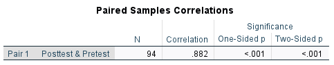
The Paired Samples Correlation table examines the relationships between the pre and post-test scores. As expected, the two scores show a strong positive correlation (r = .882, p<.001). We will cover more details about measures of association in Week 1 lecture.

 

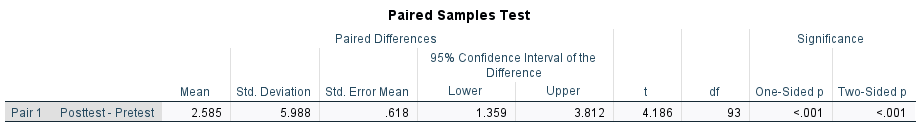
This is the key output table – Paired Sample t Test.

Mean: The average differences between the two grouping variables (2.59).

Standard Deviation: The standard deviation of the difference scores (6.00).

Standard error mean: Standard Deviation/square root of the sample size (denominator of the test statistics – 0.62)

95% Confidence Interval of the Difference: The confidence interval for the mean difference scores between the two groups. We are 95% confident the post and pre-test scores are between 1.36 and 3.81.

t: The test statistics for the paired t test (4.19).

df: the degrees of freedom of the test (93)

Significance (One-Sided p or Two-Sided p): The corresponding p-values of the test statistics with the df (<.001).

Step C: Results Interpretation

Based on the p-value above, we reject the null hypothesis that the difference between the average post and pre-test scores is zero. The results indicate that the motor skills after the intervention (M = 35.31, SD = 10.94) are significantly higher than motor skills before the intervention (M = 32.72, SD = 12.71), t (93) = 4.19, p < .001.