10 First Step of Four Step Modeling (Trip Generation)
Chapter Overview
The previous chapter introduces the four-step travel demand model (FSM), provides a real-world application, and outlines the data required to carry out each of the model steps. Chapter 10 focuses on the first step of the FSM, which is trip generation. This step involves predicting the total number of trips generated by each zone in a study area and the trips attracted to each zone based on their specific purpose. The chapter delves deeper into this process, providing detailed insights into the factors influencing trip generation and how they can inform transportation planning decisions. Trip generation is a function of land use, accessibility, and socioeconomic factors, such as income, race, and vehicle ownership. This chapter also illustrates how to incorporate these inputs to estimate trips generated from and attracted to each zone using regression methods, cross-classification models (tables), and rates based on activity units as specified by the Institute of Transportation Engineers (ITE). It also provides examples to demonstrate the model applications.
The essential concepts and techniques for this step, such as growth factors and calibration methods, are also discussed in this chapter.
Learning Objectives
- Explain what trip generation is and summarize what factors contribute to trip generation.
- Recognize the data components needed for trip generation estimation and ways to prepare them for estimation.
- Summarize and compare different methods for conducting trip generation estimation and ways to interpret their results
Introduction
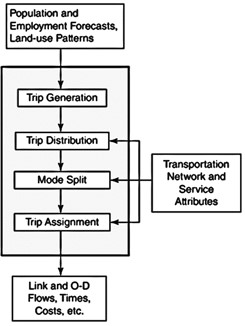
The Four-Step Model (FSM) is comprised of four consecutive steps, each addressing a specific question, ultimately contributing to an enhanced comprehension of travel demand. The questions are:
- Trip generation (Chapter 10) – How many total trips are estimated? What is the demand (total trips)?
- Trip distribution (Chapter 11) – Where are the trip destinations? What are the destinations of the trips?
- Modal split (Chapter 12) – What modes are used to complete those trips?
- Trip assignment (Chapter 13): What routes will be selected to complete the trips? (Meyer, 2016).
Figure 10.1 shows how the model is structured. It shows what kinds of data we provide as input for the model, and what steps we take to generate outputs.
Key Concepts
Link-diverted trips: Trips produced as a result of congestion near the generator and require a diversion; new traffic will be added to the streets adjacent to the site. In other words, these are trips with multiple destinations within one area and do not require road access between destinations.
Diverted trips: Travel changes in time and route are known as diverted trips. For example, when a trip is diverted or re-routed from the original travel path due to the traffic on nearby roadways, new traffic on surrounding streets results, but the trip attraction remains the same.
Pass-by trips (see below) do not include link-diverted trips.
Pass-by trips: This type of trip is described as a trip for which the destination is not a final but a stop along the way by using the connecting roads. Passing-by traffic volume in a zone depends on the type and size of development or available activities. A gas station with higher prices near an employment center may receive many pass-by trips for gas compared to other gas stations (Where up to 50 % of all trips to a service station are travelers passing by rather than people who made a special trip to the gas station)
A gas station located in close proximity to an employment center and charging higher prices might experience a higher number of pass-by trips for gas, in contrast to other gas stations. It is observed that up to 50% of all trips to a service station are by travelers passing by, rather than individuals specifically making a deliberate trip to that gas station. (Meyer, 2016).
Traditional FSM Zonal Analysis : After inputting the required data for the model, FSM calculates the number of trips generated by or attracted to each zone using the primary input using data from travel surveys from census data. While one limitation of the trip generation model is reduced accuracy due to aggregated data, the model offers a straightforward and easily accessible set of data requirements. Typically, by utilizing basic socio-economic information like population, job figures, vehicle availability, income, and similar metrics, one can calculate trip generation and distribution.
Activity-based Analysis: There are also other (newer) methods for travel demand modeling in which individual trips are modeled based on individuals’ behaviors and activities in a disaggregated manner. The methods that use activity-based models can estimate travel demand based on a basic premise—the demand to accomplish personal activities during the day (for example, work, school, personal business, and so forth) produces a demand for travel that is often connected (Glickman et al., 2015). However, activity-based models have extensive data requirements as individuals, rather than traffic analysis zones, are the unit of analysis. Detailed information on each individual’s daily activity and socioeconomic information is needed.
Travel diaries (tours) are one source of such information (Ettema et al., 1996; Malayath & Verma, 2013). Because of travel demand modeling, additional information can be learned about the study area. For example, the detailed data may reveal information about areas with or without minimum accessibility, underserved populations, transportation inequity, or congested corridors (Park et al., 2020).
Several scholars have compared the two models – traditional zonal models and activity-based models – to assess factors such as forecasting ability, accuracy, and policy sensitivity. Despite initial expectations, the findings from some studies show no improvement in the accuracy of activity-based models over traditional models (Ferdous et al., 2011). However, considering the complexity of decision-making, activity-based models can be used to minimize the unrealistic assumptions and aggregation bias inherent in FSM models. Still, the applicability and accuracy of activity-based models should be independently assessed for each context analysis to determine which is the most effective approach.
In transportation analysis, trips are typically classified based on the origin (O)and destination (D) location. As mentioned in previous sections, for a more accurate and better estimation of trip generation results, it would be better to identify a wide range of trip categories and have disaggregate results by trip purposes. The following lists typical trip classifications:
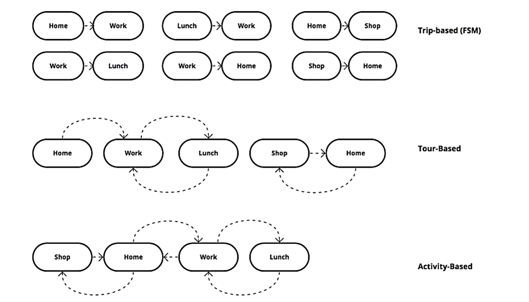
- Home-based work (HBW): If one of the trip origins is home and the destination is the workplace, then we can define the trip purpose as home-based work (HBW). These trips usually happen in the morning (to work) and in the evening (from work to home).
- Home-based non-work (HBNW): If from the two ends of the trips, one is home and the other one is not workplace, the trip purpose is home-based-non-work (HBNW). Sometimes this trip purpose is called home-se is called home-based other (HBO). Examples of these are going to services like a restaurant or hospital.
- Non-home-based (NHB): If neither the origin nor the destination is home, we can classify the trip as a non-home-based (NHB) purpose. One typical example is a lunch break trip from the workplace to a shopping mall.
While the above categories include only one origin and one destination, most individual trips are more complex due to chaining different trips into one tour. For instance, a person may stop for coffee or drop their child at daycare on the way to work, leave on lunch break for shopping, and then pick up their child from daycare on the way home. A tour is a continuous chain of trips an individual takes daily to complete their chores, which activity-based models can simulate (Ben-Akiva & Bowman, 1998). Figure 10.2 illustrates the different trip purposes and differences between FSM and activity-based models in trip classification.
It is important to note that home-based trips can be work, school, shopping, recreational, and others. While the first two are usually mandatory and made daily, the rest are less regular or discretionary.
Trips can also be classified based on the time of day that they are generated or attracted, as traffic volumes on various corridors vary throughout the day. Essentially, the proportion of different trip purposes in the total trips is more pronounced during specific times of the day, usually categorized as peak and off-peak hours (Alkaissi, 2021).
Lastly, another factor to consider is the socio-economic characteristics and behaviors of the trip makers. An understanding of these factors is crucial for classifying trips, as some possess significant influence on travel behavior (Giuliano, 2003; Jahanshahi et al., 2009; Mauch & Taylor, 1997), such as, income level, car ownership, and household size.
Trip generation
Recall from the previous chapter, a comprehensive analysis of travel demand should include trip generation and attractions for different zones. These values should be balanced to produce an equal number of trips. In general, trip generation helps predict the number of trips for different purposes generated by and attracted to every zone in a study area.
Additionally, the number of trip ends – the total number of trips entering and leaving a specific land use or site over a designated period – can be calculated in the trip generation step (New Jersey Transit, 1994). Despite recent trends for remote work, most people do not live and work in the same area. Daily round trips to work or shopping centers originate from different locations. In this regard, the distribution of activities, like job centers, can help us to understand daily travel patterns (Wang & Hofe, 2020).
After generating an overview of the distribution of activities and land uses, we must identify the factors or conditions affecting trip generation. Over the years, studies have examined factors that are now accepted as standard: income, auto ownership, family size, or density (Ewingetal.,1996;Sharpeetal.,1958).Using a zonal level analysis, population, number of jobs, and availability of modes can affect trip generation (Wang&Hofe,2020). Similarly, the type and size of retailstores can also affect the number of trips.
Additionally, the predominant travel mode chosen by the population for their daily trips is a vital factor to consider. Because of the interconnectedness of land use and transportation, the primary mode influences the distribution of services, employment centers, and the overall structure and boundaries of the city. In summary, the type and intensity of land use in combination with transportation mode play crucial roles in trip generation.
The table below shows 5 hypothetical cities where the predominant mode of transportation is different for each case. According to the speed of each mode, the extent to which activities are dispersed, determines the size of the city. For instance, a city where rail is the frequent mode of transportation, the speed (21 mph) and travel time (43 mins), the catchment (distance) would be 12 miles. Using this distance as a radius, we can estimate the size of the city.
Table 10.1 Hypothetical cities with different transportation modes
| blank cell | Speed (mph) | Time (min) | Distance (mile) | Size of the City (mile) |
|---|---|---|---|---|
| Bus | 14 | 55 | 7.5 | ? |
| Rail | 21 | 42 | 12 | ? |
| Car | 30-60 | 25 | 12.5-25 | ? |
| Bike | 8 | 15 | 2 | ? |
| Walk | 2 | 12 | 0.4 | ? |
According to the discussion here, the following categories can be identified as contributors to trip generation (McNally, 2007).
- Land-use types
- Land-use Intensity
- Location/accessibility
- Travel time
- Travel mode (transit, auto, walking …)
- Households’ income level
- Auto ownership rate
- Workers per household
Trip Generation Calibration
Traffic Analysis Zones (TAZs) connected by transportation networks and facilities are used to model the study area. TAZs are the smallest units of analysis in FSM. They are typically bounded by transportation networks or natural boundaries such as rivers.
Prior to estimating trip generators and attractions, calibrate the model as follows:
- Determine the regional population and the employment rate for the forecasting year to estimate the total number of interactions and possible future patterns.
- Allocate population and economic activities to each TAZ to prepare the study area for the modeling framework.
- Specify the significant variables and a proper method for creating the travel demand model (trip generation step). This step can be called model specification.
Calibration is an essential process in travel demand modeling. It involves collecting actual traffic flow data and calculating model parameters to verify the accuracy of the model for a specific region. The purpose of calibration is to match predicted outcomes with observed data, ensuring that model results are reliable and trustworthy (Wang & Hofe, 2020).
FSM MODELING UNITS
As discussed previously, the unit of analysis used for the model varies by model type. The unit of analysis is important as it guides data collection. Traditional zonal analysis, like FSM, typically uses TAZs. Activity-based models typically use data at the level of the individual person or household. There are three general methods for trip generation estimations:
- Growth factor model,
- regression methods,
- cross-classification models (tables),
- and rates based on activity units (ITE).
Generally, the trip generation step requires two types of data – household-based and zonal-based. Household-based data is more suitable for cross-classification analysis, and zonal-based data is more applicable for regression method analysis (the following sections will discuss these methods).
The third method is based on rates by which each land use type generates trips. The very general process for this method is identifying land use types, estimating trip generation according to ITE manuals, calculate total generation, and finally modifying based on specific characteristics such as proximity or location of land use. In this chapter, we do not wish to illustrate the third model, instead we focus on regression and cross-classification models since they are more data-oriented methods, more realistic and more frequently used in real-world.
The zonal analysis consists of areas divided into smaller units (zones), from which an estimate of trips generated in each zone is obtained (aggregate model). Household-based analysis decomposes zones into smaller units based on households with similar characteristics. In transportation travel demand modeling, we estimate zonal trips for various purposes, such as work, school, shopping, and social or recreational trips. As said, a zone is an area with homogeneous characteristics of land use, population, income, vehicle ownership, and the same access path outside of the zone.
In many cases, however, sufficient data at this resolution is unavailable (available at Census Tracts, Blocks, and Block Groups). In these conditions, the modeler should assess if the lower-resolution data is sufficient for their purpose. If not, using appropriate GIS-based data conversion methods, the data from a higher level (such as Census Tract) can be migrated to lower-level units (such as TAZ).
GROWTH FACTOR MODELING
A straightforward approach for estimating future trip generation volumes is to translate trends from the past into the future based on a linear growth trend of effective factors such as population or income. This method projects past data into the future by assuming a constant growth rate between two historical points. We can use this method when trip production and attraction in the base year are available, but the cost function (like travel time) is not. While this method is commonly used, it is important to note that it is insensitive to the distance between zones, which affects the estimated future data (Meyer, 2016).
In this model, the future number of trips equals the number of current trips times the growth factor.
Equation below is the method’s mathematical format:

where:
Ti is the number of trips in the zone in the forecasting year
ti is the current number of trips in that zone
fi is a growth factor
The growth factor itself consists of a number of explanatory variables that we acknowledge have impact on trip generation such as population, income (I), and ownership (V). To calculate a single growth factor with all these variables, the below equation is useful:

where:
Pi d is the population in the design year
Pi c is the population in the current year
Ii d is the income level in the design year
Ii c is the income level in the current year
Vi d is the vehicle ownership rate in the design year
Vi c is the vehicle ownership rate in the current year
Example 1
In a small neighborhood, 630 households reside, out of which 300 households have cars and 330 are without cars. Assuming population and income remain constant, and all households have one car in the forecasting year, calculate the total trips generated in the forecasting year and the growth factor (trip generation rate for 1-car: 2.8; 0-car:1.1). Assume that a zone has 275 households with cars and 275 without cars, and the average trip generation rates for the two groups are 5.0 and 2.5 trips per day.
Assuming all households will have a car in the future, find the growth factor and the future generated trips from that zone, keeping population and income constant.
Solution:
- Current trip rate ti=300 × 2.8 + 330 × 1.1 = ? (Trips/day)
- Growth factor Fi=Vdi/Vc =630/300= ?
- Number of future trips Ti = Fiti = 2.1 × 1203 = ? (Trips / day)
Regression Analysis
Regression analysis begins with the classification of populations or zones using the socio-economic data of different groups (like low-income, middle-income, and high-income households). Trip generation can be calculated for each category and the total generated trips by each socio-economic group such as income groups and auto ownership groups using linear regression modeling. The reason for disaggregating different trip making groups is that as we discussed, travel behavior can significantly vary based on income, vehicle availability and other capabilities. Thus, in order to generate accurate trip generations using linear models such as OLS (Ordinary Least Squares) regression, we have to develop different models with different trip making rates and multipliers for different groups. This classification is also employed in cross-classification models, which is discussed next. While the initial process for regression analysis is similar to cross-classification models, one should not confuse the two methods, as the regression models attempts to fit the data to a linear model to estimate trip generation, while cross-classification disaggregates the study area based on characteristics using curves and then attributes trips to each group without building predictive models.
Alternatively, the number of total trips attracted to each zone would be determined using regression analysis on employment data and land-use attraction rates. The coefficients for the prediction model in linear regression analysis can be derived. The prediction model has a zone’s trip production or attraction as a dependent variable, and independent variables are socio-economic data aggregated by zone. Below, we illustrate a general formula for the regression type analysis:
Trip Production= f (median family income, residential density, mean number of automobiles per household)
The estimation method in this regression analysis is OLS (Ordinary Least Squares). After zonal variable data for the entire study area are collected, linear regression analysis is applied to derive the coefficients for the prediction model. A major shortcoming associated with this model is that aggregate data may not reflect the precise effect of data on trip production. For instance, individuals in two zones with an identical vehicle ownership rate may have very different access levels to private cars, thus having different trip productions. The cross-classification model described in the next section helps address this limitation (McNally, 2007).
Equation below shows the typical mathematical format of the trip generation regression model:

where Xi is the independent variable and ai is the associated coefficient.
Example 2
In a residential zone, trip production is assumed to be explained by the vehicle ownership rate of households. For each household type, the trip-making rates are shown in Table 10.2). Using this information, derive a fitted line. Table 10.2 documents 12 data points. Each corresponds to one family and the number of trips per day. For instance, for a 1-vehicle family, we have (1,1) (1,3), and (1,4).
Table 10.2 Sample vehicle ownership data for trip generation
| Vehicle Ownership | 1 | 2 | 3 | 4 |
|---|---|---|---|---|
| Trips per day (y) | 1 | 2 | 5 | 7 |
| 1 | 3 | 4 | 5 | |
| 3 | 4 | 5 | 8 | |
| 3 | 5 | 7 | 8 | |
| Total Trips | 8 | 14 | 21 | 28 |
The linear equation will have the form: y = bx + a.
Where: y is the trip rate, and x is the household vehicle ownership, and a and b are the coefficients. For a best fit, b is given by the equation:


Based on the input table, we have:
Σx = 3 × 1 + 3 × 1 + 3 × 3 + 3 × 3 = 24
Σx2 = 3 × (12) + 3 × (22) + 3 × (32) + 3 × (42) = 90
Σy = 8 + 14 + 21 + 28 = 71
Σxy = 1 × 1 + 1 × 1 + 1 × 3 + 1 × 3 + 2 × 2 + 2 × 3 + 2 × 4 + 2 × 5 + 3 × 5 + 3 × 4 + 3 × 5 + 3 × 7 + 4 × 7 + 4 × 5 + 4 × 8 + 4 × 8 = 211
y‾ = 71/12 = 5.91
x‾ = 30/12 = 2.5
b = (nΣxy − ΣxΣy)/[(nΣx2 − (Σx)2]
=((16 × 211) − (24 × 71))/((16 × 90) − (24)2) = 1.93
a = y‾ − b x‾ = 17.75 – 1.93 × 2.5 = 12.925
y= 1.93X + 12.925
Cross Classification Models
This type of model estimates trip generation by classifying households into zones based on similarities in socio-economic attributes such as income level or auto ownership rate. Since the estimated values are separate for each group or category of households, this model aligns with our presumption that households with similar characteristics are likely to have similar travel patterns (Mathew & Rao, 2006). The first step in this approach is to disaggregate the data based on household characteristics and then calculate trip generations for each class. Aggregate all calculated rates together in the final step to generate total zonal trip generations. Typically, there are three to four variables for household classification, and each variable includes a few discrete categories. This model’s standard variables or attributes are income categories, auto ownership, trip rate/auto, and trip purpose.
The cross-classification method involves grouping households based on different characteristics such as income and family size. For each group, the trip generation rate can be calculated by dividing the total number of trips made by families in that group by the total number of households in that group within each zone (Aloc & Amar, 2013).
The following are some of the advantages of the cross-classification model:
- Groupings are independent of the TAZ system of the study area.
- No need to assume linearity as it disaggregates the data.
- It can be used for modal split.
- It is simple to run and understand. Furthermore, some of the model’s disadvantages are:
- It does not permit extrapolation beyond its calibration strata.
- No measure of goodness of fit is identifiable.
- It requires large sample sizes (25 households per cell); otherwise, cell values will vary.
After exploring the general definitions and features of the cross-classification model for trip generation estimations, we present a specific example and show how to perform each model step in detail.
Example
Suppose there is a TAZ that contains 500 households, and the average income for this TAZ is
$35000. We are to develop the family of cross-classification curves and determine the number of trips produced by purpose. The low, medium, and high income are $15,000, $25,000, and $55,000, respectively (Note: this data is extracted from 1990 and is therefore out of date. Current rates for income categories may be higher.) (Adapted from: NHI, 2005). For the first step, we should develop the family of cross-class curves for the income levels and find the number of households in each income category.
If we divide the households by six income ranges, we have the table below, derived from the survey.
Based on this table, we can plot the curves in the following format:
| blank cell | Income Category Percentages | ||
|---|---|---|---|
| Income ($000) | High | Medium | Low |
| 10 | 0 | 30 | 70 |
| 20 | 0 | 50 | 50 |
| 30 | 10 | 70 | 20 |
| 40 | 20 | 75 | 5 |
| 50 | 50 | 50 | 0 |
| 60 | 70 | 30 | 0 |
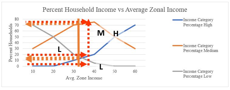
If you look at the vertical line on the $40,000 income level, you can find that the intersection of this line with three income range categories shows the percentage of households in that range. Thus, to find the number of total households in each group we have to find the intersection of the curves with average income level ($35,000). In the above plot, the orange line shows these three values, and the table below can be generated according to that:
| Income ($000) | Households (%) | HH/Zone | Total HH |
|---|---|---|---|
| Under 20 | 13 | 500 | 65 |
| 20-45 | 72 | 500 | 360 |
| 45-60 | 15 | 500 | 75 |
| 100 | 500 |
2. In the second step, after deriving the number of households in each income category, we follow the same procedure for other variables: vehicle ownership. In other words, now we find trips per household in each auto ownership/income group “class.” Again, from the survey, we have the following table, and we can generate the plot of the curves according to that:
| blank cell | Auto/HH(%) | |||
|---|---|---|---|---|
| Income ($000) | 0 | 1 | 2 | 3 |
| 10 | 48 | 48 | 4 | 0 |
| 20 | 4 | 72 | 24 | 0 |
| 30 | 2 | 53 | 40 | 5 |
| 40 | 1 | 32 | 52 | 15 |
| 50 | 0 | 19 | 56 | 25 |
| 60 | 0 | 10 | 60 | 30 |
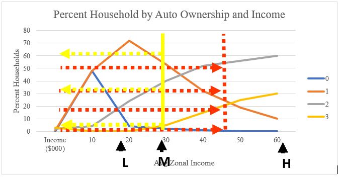
Like the previous step, the intersection of four auto ownership curves with low, medium, and high-income level lines determine the share of each auto ownership rate in each income level group:
| Percentage of HH owning # vehicles | < | < | < |
|---|---|---|---|
| Auto Ownership | Low | Medium | High |
| 0 | 26 | 3 | 0 |
| 1 | 60 | 63 | 15 |
| 2 | 14 | 32 | 58 |
| 3 | 0 | 2 | 27 |
| 100 | 100 | 100 |
3. After calculating the number of households in each income level category and auto ownership rate, the next step in the trip generation estimation procedure is to find the number of trips per household based on income level and auto ownership rate. The table below shows the trip generation rate for different income levels:
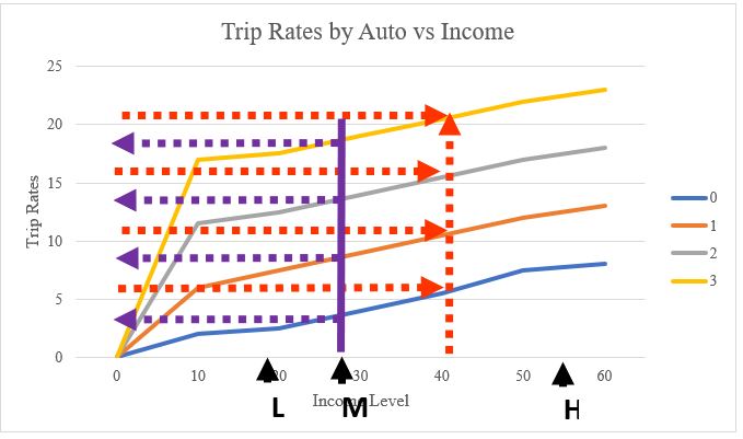
In Figure 10.3, the meeting point of three income levels and auto ownership status with trip rates yields us the following table:
| Trips per HH by Income and Auto Ownership | |||
|---|---|---|---|
| Auto Ownership | Low | Medium | High |
| 0 | 2 | 3 | 7 |
| 1 | 7 | 8 | 13 |
| 2 | 12 | 13 | 18 |
| 3 | 17 | 18 | 23 |
4. In the fourth step, we must incorporate the trip purpose into the model. To that end, we have trip purposes ratios based on income level from the survey. Like the previous steps, we plot the table on a graph to visualize the curves and find the intersection points of the curves with our three low, medium, and high-income levels:
| blank cell | Trips (%) | ||
|---|---|---|---|
| Income ($000) | HBW | HBO | NHB |
| 10 | 38 | 34 | 28 |
| 20 | 38 | 34 | 28 |
| 30 | 35 | 34 | 31 |
| 40 | 27 | 35 | 38 |
| 50 | 20 | 37 | 43 |
| 60 | 16 | 40 | 44 |
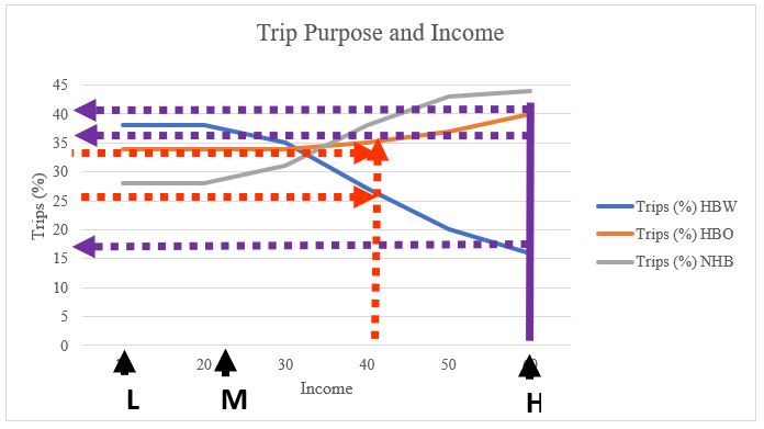
Based on the findings of this plot, we can now generate the table below, in which the percentage of trips by purpose and income level is illustrated:
| Trips per HH by Income and Trip Purpose | |||
|---|---|---|---|
| Trip Purpose | Low | Medium | High |
| HBW | 38 | 37 | 18 |
| HBO | 34 | 34 | 38 |
| NHB | 28 | 29 | 44 |
| Total | 100 | 100 | 100 |
Now, we have all the information we need for calculating the total number of trips by household income level and trip purpose.5.
5. In the next step, we calculate the total number of households in each income group based on the number of cars they own. Multiplying the number of households in each income group (00) to the percent of families with a certain number of cars (A) will give us the mentioned results.
| Income ($000) | Households (%) | HH/Zone | Total HH |
|---|---|---|---|
| Under 20 | 13 | 500 | 65 |
| 20-45 | 72 | 500 | 360 |
| 45-60 | 15 | 500 | 75 |
| 100 | 500 |
| Percentage of HH owning # vehicles | |||
|---|---|---|---|
| Auto Ownership | Low | Medium | High |
| 0 | 26 | 3 | 0 |
| 1 | 60 | 63 | 15 |
| 2 | 14 | 32 | 58 |
| 3 | 0 | 2 | 27 |
| 100 | 100 | 100 |
6. Once we have the total number of households in each group of income based on auto ownership, we multiply the results to the trips rate (B) so that we have the total number of trips for each group.
| Trips per HH by Income and Auto Ownership | |||
|---|---|---|---|
| Auto Ownership | Low | Medium | High |
| 0 | 2 | 3 | 7 |
| 1 | 7 | 8 | 13 |
| 2 | 12 | 13 | 18 |
| 3 | 17 | 18 | 23 |
| Number of HH owning # vehicles | |||
|---|---|---|---|
| Auto Ownership | Low | Medium | High |
| 0 | 17 | 11 | 0 |
| 1 | 39 | 227 | 11 |
| 2 | 9 | 115 | 44 |
| 3 | 0 | 7 | 20 |
| 65 | 360 | 75 |
7. In the next step, we sum the results of the number of trips by the auto ownership number to have the total number of trips for each income group (∑(00xAxB)).
| Trips Made by Income Level | blank cell | |||
|---|---|---|---|---|
| Auto Ownership | Low | Medium | High | blank cell |
| 0 | 34 | 32 | 0 | |
| 1 | 273 | 1814 | 146 | |
| 2 | 109 | 1498 | 783 | |
| 3 | 0 | 130 | 466 | |
| 416 | 3474 | 1395 | 5285 |
| Trips per HH by Income and Trip Purpose | |||
|---|---|---|---|
| Trip Purpose | Low | Medium | High |
| HBW | 38 | 37 | 18 |
| HBO | 34 | 34 | 38 |
| NHB | 28 | 29 | 44 |
| Total | 100 | 100 | 100 |
8. Finally, the results from the above table (416, 3474, 1395) will be multiplied by the percentage of trip purposes for each income group in order to estimate the number of trips by trip purposes for each income group. The table below shows these results as the final trip generation results (example adapted from: NHI, 2005).
Cx∑(00xAxB):
| Number of Trips by Purpose | ||||
|---|---|---|---|---|
| Trip Purpose | Low | Medium | High | blank cell |
| HBW | 158 | 1285 | 251 | 1694 |
| HBO | 141 | 1181 | 530 | 1852 |
| NHB | 116 | 1007 | 614 | 1737 |
| Total | 415 | 3473 | 1395 |
Trip Attraction in the Cross-Classification Model
In the previous section, we modeled trips generated from different households and zones, and calculated their total number by purpose. However, in trip generation, trip attractions play a crucial role, along with trip production. To measure the attractiveness of zones, we can use an easy and straightforward method, which is to determine the size of each zone and the land use types within it, such as square feet of floor space or the number of employees. We can then derive trip generation rates for different attractions from surveys. Trip attractions refer to the number of trips that end in one zone. Typically, we express trip generation rates for different attractions in terms of the number of vehicle trips per household or unit area of non-residential land use. For instance, Table 10.13 provides trip attraction rates for residential and some non-residential land uses. The number 0.074 for HBW trips means that each household can attract 0.074 HBW vehicle trips per day. For non-residential land uses, the numbers are also dependent on the type and size of land uses. As shown in Table 10.13, the retail sector is more attractive than the basic sector.
Table 10.13 shows that the retail sector is more attractive than the basic sector.
| blank cell | Trip Purpose | ||
|---|---|---|---|
| Type of Activity | HBW | HBNW | NHB |
| Households (unit) | 0.074 | 0.668 | 0.412 |
| Retail (sq . km) | 139 | 419 | 332 |
| Basic (sq . km) | 122 | 84.3 | 93.8 |
After collecting the necessary data from surveys or other appropriate sources, a regression analysis can be used to determine the attraction rates for each land-use category. Then, the HBW vehicle trips attracted to a zone are then calculated as:

where:
TAHBW_H = home-based work vehicle trip attractiveness of the zone by households
Nhh = number of household in the zone
TAR_R = trip attraction rate by households
In a similar way, the HBW trips attracted by retail are calculated from the size of retail land use and the retail trip attraction rates.

where:
TAHBW_NR = home-based work vehicle trip attractiveness of the zone
A_NR = non-residential land use size in the zone
TAR_NR = trip attraction rate of the non-residential land use
Example
Assume that Table 10-14 is derived from survey data in a hypothetical city and attractiveness of each land use by trip purpose is generated.
| blank cell | Attractions per Household | Attractions per Nonretail Employee | Attractions per Downtown Retail Employee | Attractions per Other Retail Employee |
|---|---|---|---|---|
| HBW | – | 1.8 | 1.7 | 2 |
| HBO | 1.3 | 2.2 | 5.4 | 9 |
| NHB | 1 | 1.1 | 3 | 5.1 |
Additionally, a new retail center in a part of the city accommodates 370 retail workers and 550 non-retail workers. According to this information, the number of trips attracted to this area can be calculated as:
First, using the information in table 10.14:
HBW: (370 * 1.7) + (550 * 1.8) = 1619
HBO: (370 * 5.4) + (550 * 2.2) = 3208
NHB: (370 * 3.0) + (550 * 1.1) = 1715
Total = 6542trips/day (example adopted from: Alkaissi, 2021)
Balancing Attractions and Productions
After generating trips, the final step is to balance trip production and attraction. Since trip generation is more accurate, and its validity is more reliable compared to trip attraction models, attraction results are usually brought to the scale of trip generation. Balance factors are used to balance Home-Based Work (HBW) trip attraction and production, which is illustrated in the example below.
| blank cell | Unbalanced HBW Trips | Balanced HBW Trips | ||
|---|---|---|---|---|
| Zone | Productions | Attractions | Productions | Attractions |
| 1 | 150 | 260 | 150 | 195 |
| 2 | 250 | 380 | 250 | 285 |
| 3 | 200 | 160 | 200 | 120 |
| Total | 600 | 800 | 600 | 600 |
According to Table 10.15, the total number of trips generated by all three zones is 600. However, the total number of trips attracted to all the zones is 800, which is an unreasonable value. To fix this issue, we use a balancing factor to multiply each cell in the attraction column by (600/800).
When planning NHB (non-home-based) trips, it is important to take an extra step to ensure that the production and attraction outputs are balanced. This means that for all zones and each zone, the total number of trips attracted and generated should be the same. The reason for this is that NHB trips have unknown origins, meaning that the origin information is not available through surveys or census data. Therefore, the most accurate estimate possible is to set the total NHB productions and attractions to be equal.
Conclusion
In this chapter, we introduced and reviewed the first step of travel demand modeling that is developed for estimating trip generation from each neighborhood or zone. We specifically focused on different methods (growth factor, regression, and cross-classification) and provided examples for each method along with an overview of key concepts and factors contributing to trip generation. Today, the ongoing advancements in computational capacity as well as capabilities for real-time data collection appear to be promising in equipping us with more accurate predictions of trip generation. For instance, GPS mobile data can be used to empirically estimate the rate of trip generation, build advanced models (such as machine learning models) to develop highly calibrated and optimized models.
In the next chapter, we learn about trip distribution. It is worth noting here that the trip distribution is completely based on a foundation of attractiveness of various location determined in trip generation step. As we will see, we used gravity-based models to allocate demand to pair of zones in space. In other words, four-step model is a sequential model, in which the accuracy and reliability of the each step depends on model performance in previous steps.
Glossary
- activity-based model is travel forecasting framework which is based on the principle that travel is derived from demand reflected in activity patterns of individuals.
- Travel diaries (tours) refers to a chain of trips between multiple locations and for different purposes such as home to work to shopping to home.
- Land-use Intensity is a measure of the amount of development on a piece of land usually quantified as dwelling per acre.
- Pass-by trips refers to the trips for which the destination is not a final destination but rather an stop along the way by using the connecting roads.
- Diverted link trips are produced from the traffic flow in the adjacent area of the trip generator that needs diversion. This new traffic will be accumulated in the roadways close to the site.
Key Takeaways
In this chapter, we covered:
- What trip generation is and what factors influence trip generation.
- Different approaches for estimating trip generation rates and the data components needed for each.
- The advantages and disadvantages of different methods and assumptions in trip generation.
- How to perform a trip generation estimation manually using input data.
Prep/quiz/assessments
- List all the factors that affect trip generation. What approaches can help incorporate these factors?
- What are the different categories of trip purposes? How do newer (activity-based models) models differ from traditional models (FSM) based on trip purposes?
- What are the data requirements for the growth factor model, and what shortcomings does this method have?
- Why should trip productions’ and attractions’ total be equal, and how do we address a mismatch?
References
Alkaissi, Z. (2021). Trip generation model. In Advanced Transportation Planning, Lecture, 4. Mustansiriya University https://uomustansiriyah.edu.iq/media/lectures/5/5_2021_05_17!10_34_51_PM.pdf
Aloc, D. S., & Amar, J. A. C. (2013). Trip generation modelling of Lipa City. Seminar and research methods in civil engineering research program, University of Philippines Diliman. https://doi.org/10.13140/2.1.2171.7126.
Ben-Akiva, M.E., Bowman, J.L. (1998). Activity based travel demand model systems. In: P. Marcotte, S. Nguyen, S. (eds) Equilibrium and advanced transportation modelling. Centre for Research on Transportation. Springer, Boston, MA. Kluwer Academic Publishers, pp. 27–46. https://doi.org/10.1007/978-1-4615-5757-9_2
Ettema, D., Borgers, A., & Timmermans, H. (1996). SMASH (Simulation model of activity scheduling heuristics): Some simulations. Transportation Research Record, 1551(1), 88–94. https://doi.org/10.1177/0361198196155100112
Ewing, R., DeAnna, M., & Li, S.-C. (1996). Land use impacts on trip generation rates. Transportation Research Record, 1518(1), 1–6. https://doi.org/10.1177/0361198196151800101
Giuliano, G. (2003). Travel, location and race/ethnicity. Transportation Research Part A: Policy and Practice, 37(4), 351–372. https://doi.org/10.1016/S0965-8564(02)00020-4
Glickman, I., Ishaq, R., Katoshevski-Cavari, R., & Shiftan, Y. (2015). Integrating activity-based travel-demand models with land-use and other long-term lifestyle decisions. Journal of Transport and Land Use, 8(3), 71–93. https://doi.org/10.5198/jtlu.2015.658
ITE, I. of T. E. (2017). Trip generation manual. ITE Journal. ISSN 0162-8178. 91(10)
Jahanshahi, K., Williams, I., & Hao, X. (2009). Understanding travel behaviour and factors affecting trip rates. In European Transport Conference, Netherlands (Vol. 2009). https://www.researchgate.net/profile/Kaveh Jahanshahi/publication/281464452_Understanding_Travel_Behaviour_and_Factors_Affecting_Trip_Rates/links/57286bc808ae262228b5e362/Understanding-Travel-Behaviour-and-Factors-Affecting-Trip-Rates.pdf
Malayath, M., & Verma, A. (2013). Activity based travel demand models as a tool for evaluating sustainable transportation policies. Research in Transportation Economics, 38(1), 45–66. https://doi.org/10.1016/j.retrec.2012.05.010
Mathew, T. V., & Rao, K. K. (2006). Introduction to transportation engineering. Civil Engineering–Transportation Engineering. IIT Bombay, NPTEL ONLINE, https://www.civil.iitb.ac.in/tvm/2802-latex/demo/tptnEngg.pdf
Mauch, M., & Taylor, B. D. (1997). Gender, race, and travel behavior: Analysis of household-serving travel and commuting in San Francisco bay area. Transportation Research Record, 1607(1), 147–153.
McNally, M. G. (2007). The four step model. In D. A. Hensher, & K. J. Button (Eds.), Handbook of transport modelling, Volume1 (pp.35–53). Bingley, UK: Emerald Publishing. http://worldcat.org/isbn/0080435947
Meyer, M. D., (2016). Transportation planning handbook. John Wiley & Sons: Hoboken, NJ, USA, 2016.
New Jersey Transit, N. (1994). Planning for transit-friendly land use: A handbook for New Jersey communities. NJ Transit, Trenton, NJ.
NHI. (2005). Introduction to Urban Travel Demand Forecasting. In National Highway Administration (Ed.), Introduction to Urban Travel Demand Forecasting. American University. National Highway Institute : Search for Courses (dot.gov)
Park, K., Sabouri, S., Lyons, T., Tian, G., & Ewing, R. (2020). Intrazonal or interzonal? Improving intrazonal travel forecast in a four-step travel demand model. Transportation, 47(5), 2087–2108. https://doi.org/10.3141/1607-20
Sharpe, G. B., Hansen, W. G., & Hamner, L. B. (1958). Factors affecting trip generation of residential land-use areas. Highway Research Board Bulletin, 203. http://onlinepubs.trb.org/Onlinepubs/hrbbulletin/203/203-002.pdf
Wang, X., & Vom Hofe, R. (2020). Selected methods of planning analysis (2nd ed. 2020 edition). Springer. Springer Nature. https://doi.org/10.1007/978-981-15-2826-2
Whitney, V. (2019, September, 29). Activity & Trip Based Travel Models. Medium. https://medium.com/data-mining-the-city/activity-trip-based-travel-models-e4833571570
Land-use Intensity is a measure of the amount of development on a piece of land usually quantified as dwelling per acre.
Cross-classification is a method for trip production estimation that disaggregates trip rates in an extended format for different categories of trips like home-based trips or non-home-based trips and different attributes of households such as car ownership or income.
