3 An Overview of the Integrated Land-Use Transportation Modeling Process
Chapter Overview
This chapter provides a detailed discussion about interactions, forces, and relationships between land use change and transportation, along with the ways scholars have understood and conceptualized this relationship. To do this, the chapter goes back to theories of the 19th century and identifies the initial attempts in defining or modeling urban structure based on transportation costs and land market. The chapter also goes over the most prominent US-centered theories of urban from of 20th century such as sector model or concentric zones to charter the way our understanding about evolution of cities has shaped over time. The chapters also explain why and how accessibility is at the heart of land use/transportation models and progresses to identify the major components of land use/transportation models. Finally, the chapter provides a timeline of different modeling approaches and a recap of how these approaches compare to one another.
Learning Objectives
- Explain the way land use and transportation interact and factors affecting this interactions.
- Illustrate the feedback loop between the land use and transportation with intervening features.
- Describe theories, key indicators, and components of land-use transportation models.
- Identify the initial models of land-use transportation models and their impact on current models.
- Recognize and compare different approaches of current land-use transportation modeling framework
Introduction
This chapter delves into the dynamics of land use and transportation interactions and the models that best represent them, introducing fundamental concepts before delving into more detailed models in subsequent chapters. While comprehensive discussions of specific models will be presented later, this chapter lays the groundwork for understanding the basics of these interaction models.
Throughout history, various factors have played a role in influencing the location of activities and land uses, with transportation costs emerging as a pivotal factor. Land-use decisions, whether for residential, commercial, or industrial purposes, are often driven by the aim of minimizing transportation costs. The twentieth century witnessed the development of numerous models and theories concerning transportation costs and land-use determination. Models, serving as abstract reflections of real-world conditions, include theories like concentric zones, theory of axial development, and agricultural land rent theory. The models discussed in this book provide insights into explaining and predicting land-use patterns in many American contexts. According to these models, most cities have evolved around a hub-and-spoke transportation infrastructure, so the central urban area houses high-rent paying activities. As activities are located further away from the center, land rents decrease (Hensher, 2004).
Thus, land use and transportation have an ever-ongoing interaction with each other. Transportation professionals consider the circumstances and the extent to which transportation projects and implementation practices induce variations in urban form and development. Location choices are another consideration dependent on the accessibility of transportation systems. Recent models were developed to address these variables with the least uncertainty. In land use/transportation models, similar to any model, an abstract version of a real-world scenario is represented, leaving several types of uncertainty unaddressed.
One of the primary focuses of this book is the discussion of transportation models to help determine these uncertainties in the form of factors affecting individuals’ behaviors, owing to urban development, trip generation, and, most importantly, the decision choices of riders, drivers, operators, or agents. These agents can be individual trip makers, households who make daily trips with a recurring pattern, or economic activities who acquire land for setting up their business.
While these models are designed to simulate typical transportation features and land use conditions, their application extends to explaining global incidents and forecasting future events and trends like adoption of newer technologies such as autonomous vehicles, or impact of decisions such as affordable housing development. However, forecasting future conditions is a challenging task, and current models often exhibit inaccuracies. In urban transportation modeling, for instance, most models inevitably incorporate errors stemming from issues such as data quality and quantity, information shortages, or modeling approaches that oversimplify reality. Therefore, it is crucial to use these models with careful attention to contextual variables, their corresponding data quality, and a commitment to constant improvement (Zhou et al., 2022).
Nevertheless, despite these challenges, transportation and land-use planning models have proven beneficial in:
- Simulating interactions between land use and transportation systems.
- Estimating potential outcomes in urban systems to facilitate long-range planning.
- Supporting transportation and land-use decisions that profoundly impact people’s lives.
Transportation and Urban Form
The density and development patterns of cities, referred to as urban form, are intricately tied to the evolution and advancement of transportation systems. Understanding the relationship between transportation and urban form is essential for effective urban transportation planning, given the complexity of the relationship influenced by myriad interconnected factors within the urban context.
The initial step in the integrated modeling process involves simplifying this complex relationship by analyzing two major factors: travel demand and travel behavior. With a foundational understanding of this relationship and the identification of typical characteristics of urban form, further modeling can be developed. The interdependence of land use and transportation becomes evident, where the transportation system shapes the distribution of activities and urban form, and conversely, urban form and development type impact mode choice, mobility patterns, and the transportation network (Giuliano, 2004; Giuliano & Small, 1991; Boarnet et al., 2017; Cervero & Wu, 1997).
For example, urban density is crucial for establishing a multi-modal transport system, a feature often lacking in North American cities. The extensive post-World War II investments in interstate highway construction led to the sprawl of low-density suburbs in many cities, resulting in a loss of density supporting transit. Consequently, the evolution of transportation is closely linked to changes in urban form, manifesting in new development clusters and regional polycentric urban forms due to shifts in transportation and mobility patterns.
Furthermore, advancements in freight transport, such as containerization, have given rise to secondary employment hubs or subcenters, transforming the urban form from monocentric to polycentric. This underscores the multifaceted relationships between urban form and diverse economic driving forces (Rodrigue, 2020).
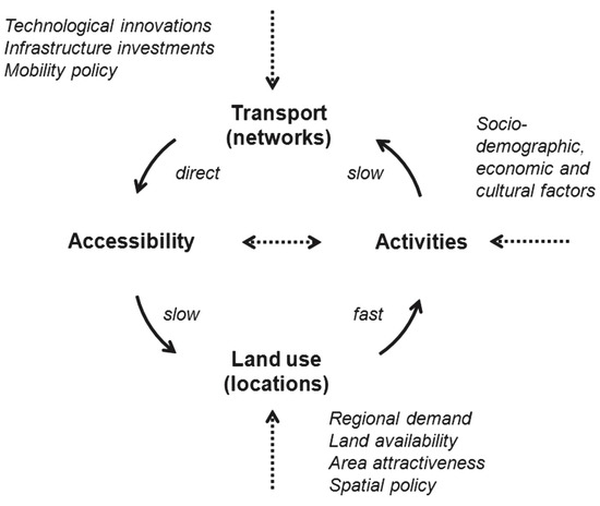
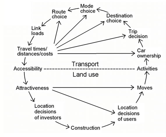
Despite these shifts, one constant factor is people’s willingness to commute for around 30-40 minutes in one direction, translating to a daily willingness to spend up to 1.2 hours commuting (Niedzielski & Kucharski, 2019). This travel behavior emphasizes a crucial component of land use and transportation analysis—accessibility. Thus, transportation significantly shapes the area’s urban limits and development and activity patterns. Figure 3.1 illustrates the general interrelation between transportation and land use, while Figure 3.2 outlines the sequential factors forming a continuous relationship between land use and transportation.
Accessibility
The spatial interaction between land use and transportation determines the land-use-transportation system, and accessibility is a measure of the ease of reach of destinations within this system (El-Geneidy & Levinson, 2006; Hansen, 1959). For instance, households prefer locations with high accessibility to jobs, schools, parks, shops, and other amenities. Similarly, businesses favor locations with high accessibility to labor, markets, customers, and more. The demand for travel is a response to the opportunities or destinations offered by the land-use transportation system. As a result, effective transportation planning should commence with land-use projections, providing essential input for the travel demand modeling process (Anjomani, 2009). Accessibility, being a comprehensive measure, encapsulates various aspects of both land use and transportation systems in a single, straightforward metric. Consequently, alterations in either land use or transportation can have a direct impact on accessibility.
Moreover, the accessibility measure utilizes data obtained through standard transportation studies and analysis (Davidson, 1977). These data should encompass an attractiveness index for the destination, like the number of jobs, a trip-making rate or emissivity index for the trip origin, such as the number of workers, and the distance between the two origins and destinations represented in terms of travel time, cost, or distance. Typically, such data is publicly available, often accessible through sources like the Census Bureau or the American Association of State Highway and Transportation Officials (ASHTO) Census Transportation Planning Products (CTPP).
In straightforward terms, land use plays a crucial role in shaping the urban form, influencing spatial interaction and transportation. Accessibility, which measures the means to reach various opportunities, is a key consideration. Consequently, transportation planning should begin with land-use projections to provide essential input for the travel demand modeling process (Anjomani, 2009). What makes accessibility powerful is its ability to combine various characteristics of both land use and transportation systems into a single, straightforward measure. This means alterations in either of these systems can directly impact accessibility.
Accessibility (A) means the ease of reaching certain activities or destinations. If a place is easily reachable from several locations or origins, it is considered highly accessible. Areas with low accessibility have fewer reachable destinations, resulting in higher travel cost and time. Hansen (1959) developed a general mathematical formula for measuring accessibility presented below:

where:
Wj is a vector of weights associated with destinations e.g. the number of jobs in a traffic analysis zone (TAZ) (j)
Cij is a cost of travel from i to j and
F(cij) is an impedance function or friction factor representing the cost, or burden (and thus utility) of a trip between the origin (i) and destination (j) for an individual.
Land-use/Transportation Modeling Framework
Transportation planners rely on current activity and land-use data as the primary input for modeling and analysis. However, these inputs are suitable only for short-term analysis, typically spanning three to five years. In such cases, an inventory of the existing land-use activity system is sufficient to estimate travel demand and mobility within the network.
While current data is effective for short-term projections, it may fall short in accurately forecasting travel demand beyond five years. This limitation arises from the dynamic nature of neighborhoods, where changes in population, employment, and the development of new areas, along with the decline or renovation of older ones, can occur. Consequently, travel demand patterns and transportation system requirements evolve over time (Meyer, 2016).
The extent and timeframe of changes in land use vary across different planning research typologies. For instance, comprehensive planning typically considers a 20-30-year timeframe, while long-range transportation planning often employs a 20-year horizon. Therefore, it is crucial to consider the timeframe when conducting integrated land-use and transportation analysis.
Failure to align land development with transportation supply and demand considerations, or vice versa, can result in unnecessary social, physical, and economic costs with fewer benefits (Miller & Soberman, 2003).
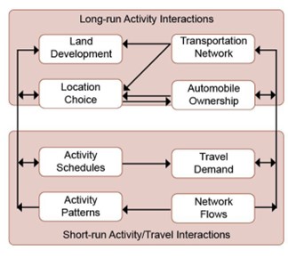
Figure 3.3 visually illustrates the components of integrated land-use and transportation planning models, distinguishing those relevant to short-term studies (3-5 years) from those typically informing long-term studies. Long-term planning models often highlight the impact of changes in the transportation network on land development. For example, the anticipation of a new road extension to the city’s outskirts could lead to the development of new subdivisions. This, in turn, would influence the locational decisions of households moving to the urban periphery, choosing to commute daily by private automobile. As a result, there could be an increase in travel demand on the roadway network serving that area of the city, potentially leading to traffic congestion and necessitating further transportation changes and investment to accommodate the new demand. To summarize, short-run activities and travel interactions are fairly linear, primarily involving activities and travel demand, while interactions over the long run are more complex and include the influence of the transportation network on land development patterns and location choice, which is also related to automobile ownership.
These models provide the likely future locations of housing, jobs, and other zonal and spatial data, predicting a study area’s growth from a series of factors, both internal (like system accessibility) and external factors (climate or economy). However, empirical research demonstrates a mutual influence between transportation systems and land-use data. Relying solely on static information for forecasting the future may yield unrealistic results.
For instance, let’s take a transportation project extending a rail line. While the model may suggest potential growth areas, the improvement in accessibility can make other neighborhoods more appealing or displace lower-income population groups. To accurately evaluate such projects, it is essential to incorporate up-to-date and dynamic socio-economic data that reflects the changing landscape of the study area.
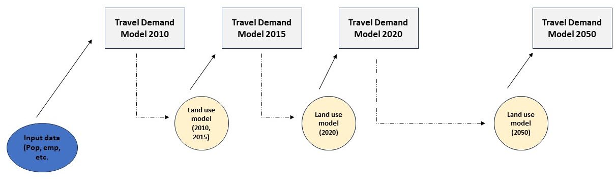
The interplay between land use and transportation does not always require a highly complex model; it can be a straightforward process. Illustrated in Figure 3.4, the model initiates the analysis with land-use information from the base year. Subsequently, the transportation model runs for the same year, generating updated travel time and costs. These outcomes are then integrated into the land-use model for the subsequent year. The output from this process replaces the base year data for the next iteration of running the transportation model.
The essence of integrated land use/transportation modeling are developed to:
- Capture the feedback cycle of land use and transportation.
- Inform decision-making and the implementation of land-use transportation projects such as smart growth & transit-oriented development.
- Assist with the analysis of greenhouse gas emissions and pricing policies.
- Regularly evaluate transport policies and their effect on location choices and tax revenue distributions.
This type of model depicts who lives where and, thus, who will receive the benefits of and who will be burdened by transport projects and thus can be a very suitable framework of transportation equity analysis. (“Travel Forecasting Resource,” 2022).
For instance, Lee et al. (2006) introduced an integrated land-use and transportation model named the Equity-based Land-Use Transportation Problem (ELUTP). This model aims to assess the distribution of travel time among network users or trip zones and the changes in equilibrium O-D (Origin-Destination) travel costs based on land use development for equity considerations. Various other applications of integrated models for diverse purposes are discussed in subsequent chapters.
Most importantly, enabling of modelers to develop equity analysis since these models determine who lives where and, thus, who will receive benefits and who will be burdened by transport projects (“Travel Forecasting Resource,” 2022).
LAND-USE/TRANSPORTATION MODELING COMPONENTS
As we discussed before, land use and transportation interactions are highly complex. Land use determines the distribution of people and economic activities as well. Spatial interaction between land use and transportation occurs when people move between locations, and the transportation system must support such movements as smoothly and conveniently as possible. Figure 3.5 shows how different transportation and land use components work together to create a system. In this figure, three main components are shown:
• Demand, represented as spatial accumulation of population, travel, etc.
• Friction, represented by the spatial separation and cost, and
• Supply represented by transport infrastructure in the form of roads, transport hubs, etc.
Since these models deal with the behavior of individuals and the movement patterns associated with their decisions, numerous components, and factors should be incorporated into the model to yield more accurate outputs. Figure 3.7 illustrates the most critical components of a model design – physical system, active agents, and processes.
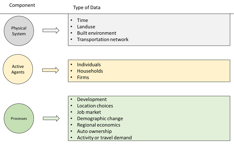
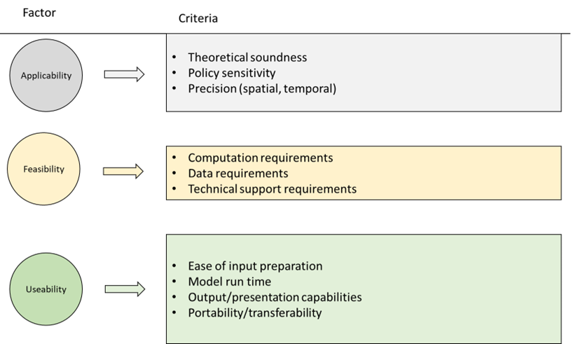
Figure 3.6, based on Hensher’s work in 2004, highlights the major factors to consider when developing a transportation and land-use model –applicability, feasibility, and usability. Evaluating these factors involves assessing their ability to yield precise and accurate results, computational capacity requirements, data availability and requirements, model running time, and the generalizability of results. The absence of these prerequisites may result in an incomplete integrated model, leading to ineffective evaluation of various scenarios or policies.
Transportation/land-use models serve as valuable tools for policymakers due to their predictive capabilities. In the 1960s and 1970s, these models primarily focused on estimating peak demand for transportation services and providing the tools and general responses necessary to meet such demands. Additionally, these models played a crucial role in evaluating the impacts of infrastructure improvements and conducting comparisons and assessments of different scenarios through cost-benefit analysis. Today, modelers in the land use transportation domain must also consider ongoing social, environmental, and economic factors.
With a return to urban lifestyles and the adoption of transportation demand management techniques that have reduced peak demand in certain urban contexts, policies now need to address the shifting times of people’s travel to non-peak hours, making the best use of existing capacity. The traditional fixed peak-hour model is becoming less relevant due to today’s increasing flexibility in non-work travel times, extended shopping hours, and business operations. Effective policies for shifting travel times may involve:
- transportation management and maintenance,
- land-use infrastructure and network improvements, and
- surveillance of supply and demand, all of which rely on accurate and reliable data and analysis.
A Brief History of Land-use Transportation Planning
The study of land-use transportation dynamics also focuses on the role of transportation facilities and networks as crucial factors in influencing land-use changes. A pioneering and widely recognized model that integrates land-use and transportation is the Lowry model (1963), which remains influential today. Several model systems, including the Desegregated Residential Allocation Model (DRAM), EMPloyment ALlocation (EMPAL), and MetroScope, have adopted Lowry’s methodologies. More advanced models using mathematical programming include the Projective Optimization Land Use Information System (POLIS) and Optimum Placement of Activities into Zones (TOPAZ).
modeling spatial interactions through input-output analysis, is another technique in land use/transportation modeling with MEPLAN and TRANUS being prominent examples, as detailed in Chapter 8. Other models, like IUSMC and CSGE, focus on economic equilibrium conditions,. The advancement of computing power has enabled large-scale microsimulation models such as MASTER, URBANSIM, TILUMIP2, and Markovian to gain attention in recent decades.
Real-world case studies of these models implemented in cities globally have led to the development of various transferable commercial packages. A common feature across these models is the consideration of accessibility to opportunities (e.g., work, shopping, home) in agents’ decision-making, influencing the dynamics of urban space and spatial distribution (Hansen, 1959; Zhang, Xu, & Li, 2009).
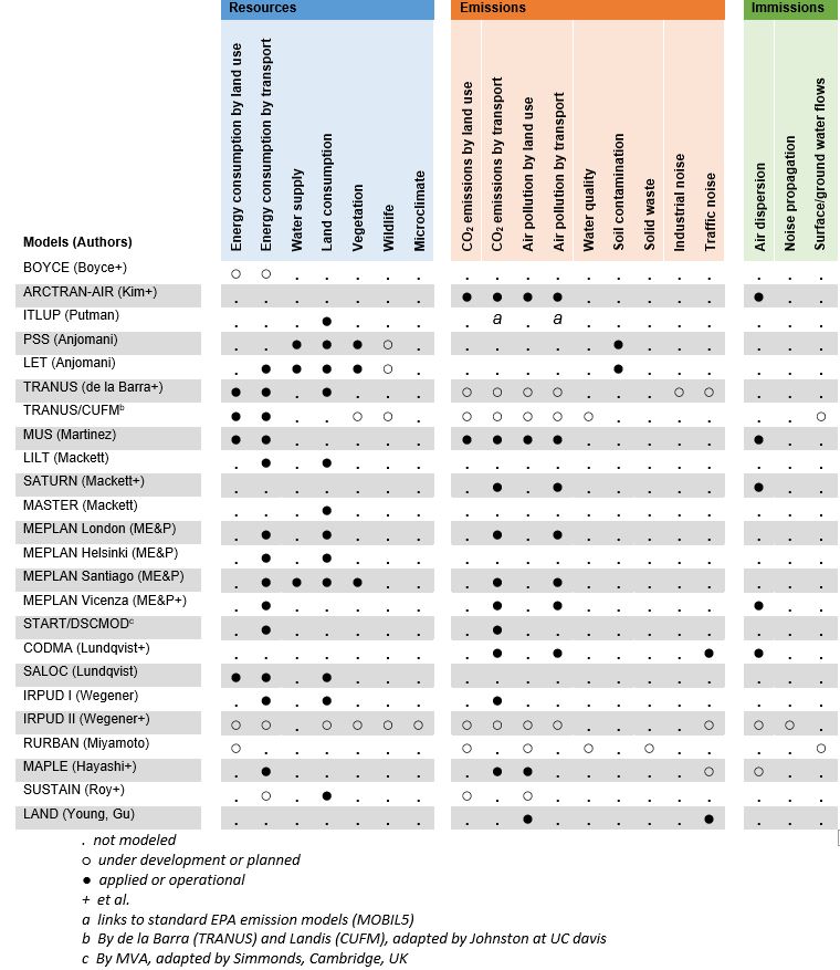
Tables 3.1 and 3.22 provide summaries of important land use/transportation models, detailing their features and applications in environmental impact assessments.
Cities and urban structures have been the subject of observation, modeling, and prediction since the 19th century. The earliest contributor to this field was Von Thünen, whose agricultural land rent theory in 1826 influenced later theories, such as the bid rent theory in a monocentric city where land price and demand decrease with distance from the city center (Clark, 1967). Christaller (1933) introduced the central place theory, a spatial geography model explaining the hierarchy and distribution of central places forming a network of marketplaces for goods with minimized overall transportation costs. Krugman (1996) contributed by conceptualizing polycentric urban forms through the study of inter-dependent location choices of agents in a metropolitan area (Zhang, Xu, & Li, 2009). Forces both centripetal and centrifugal played a role in the formation of polycentric cities. While these foundational models offer realistic predictive capabilities, they have been criticized for their oversimplification, lacking considerations of accessibility and the characteristics of the transportation network.
| Model | Subsystems modeled | Model theory | Policies modeled |
|---|---|---|---|
| POLIS composite | employment population housing land use travel | random utility locational surplus | land-use regulations transportation improvements |
| CUFM composite | population land use | location rule | land-use regulations environmental policies public facilities transportation improvements |
| BOYCE unified | employment population networks travel | random utility general equilibrium | transportation improvements |
| KIM unified | employment population networks goods transport travel | random utility bid-rent general equilibrium input-output | transportation improvements |
| METROSIM unified | all subsystems except goods transport | random utility bid-rent general equilibrium | transportation improvements travel-cost changes |
| ITLUP composite | employment population land use networks travel | random utility network equilibrium | land-use regulations transportation improvements |
| HUDS composite | employment population housing | bid-rent | housing programs |
| TRANUS composite | all subsystems | random utility bid-rent network equilibrium land-use equilibrium | land-use regulations transportation improvements transportation-cost changes |
| 5-LUT unified | population networks housing | random utility bid-rent general equilibrium | transportation improvements |
| LILT composite | all subsystems except goods transport | random utility network equilibrium land-use equilibrium | land-use regulations transportation improvements travel-cost changes |
| MEPLAN composite | all subsystems | random utility network equilibrium land-use equilibrium | land-use regulations transportation improvements transportation-cost changes |
| IRPUD composite | all subsystems except goods transport | random utility network equilibrium land-use equilibrium | land-use regulations housing programs transportation improvements travel-cost changes |
| RURBAN unified | employment population housing land use | random utility bid-rent general equilibrium | land-use regulations transportation improvements |
The following section will discuss the early land use/transportation models in more detail. We begin this section with spatial models. Spatial modeling refers to a particular form of disaggregation in which a large area comprises several smaller similar units (mostly grid squares or polygons). As discussed throughout this chapter, planning for land use in cities is a complex multiparameter challenge. Land-use decisions significantly impact several aspects of a city, such as air and water pollution, real estate, and, more importantly (for us), accessibility and travel demand. That said, scholars have developed several urban land use models characterized by different levels of complexity.
The Von Thünen Model
Von Thünen, in 1826, developed the first spatial model (Figure 3.7), which considers the city center as the primary market that affects its surrounding areas through a concentric pattern of land use. Transportation costs are the most critical variable determining the types of agricultural products in each ring. As a result, the most productive activities have the power to compete for the land closest to the central place. As activities become less productive, they choose their location further away from the center.
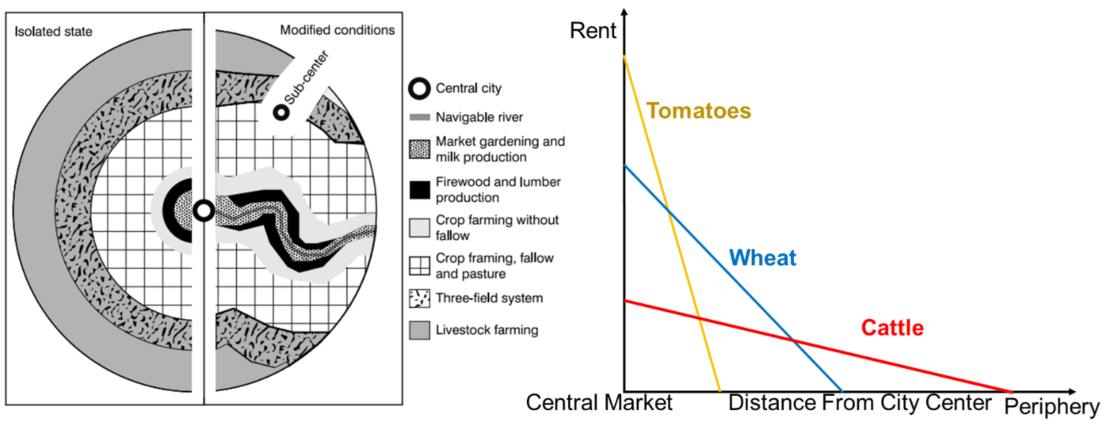
This model was developed originally based on an agrarian economy in Germany where the city is located centrally within an “isolated state” (Von Thünen, 1826) that is self-sufficient. The state or market is located on unoccupied land without geographic features. A further assumption is that farmers are looking to maximize their profit, which is a function of their transportation costs, land rent, and production types. The most significant assumption of the model, which is also seen frequently in real-world cases, is the formation of concentric rings around a market (Sharma, Sharma, & Kumar, 2011).
Von Thünen initially considered four types of products: produce, resource materials, agriculture, grazing land. Produce like fruits, vegetables, or dairy should be marketed and consumed quickly, so their production site should be close to the city center. Wood and lumber were crucial for heat and construction but were very heavy. As a result, their transport costs would be very high if they were located far from the market. Crops or grains are much more long-lasting and lighter than fruits and lumber; thus, this sector’s farmers decreased their rent by locating their establishments further away from the central market. Finally, ranching is situated in the last ring, where livestock can walk freely and occupy a more significant piece of land. Also, since they are self-transporting, their transportation costs could be meager even far from the city market. Beyond these four rings, the distance is so high that no farmer or stockman is interested in producing and selling in the market (Sinclair, 1967).
Even though Von Thünen developed his model before industrialization (before factories and railroads), it shows the trade-offs between land-use, rent, and transportation costs that create concentric ring formations around the urban core. The Von Thunen model includes the following assumptions:
- Only one market is available to farmers, at the very center of the rings.
- The land is plain, and resources are evenly distributed.
- Labor is indifferent to their work location (different rings in this case).
- Transportation and movement are possible in every direction (Euclidean network).
- Transportation costs and distance are always positively correlated.
- Farmers are rational and try to maximize their profit.
Concentric Zones
This theoretical model is a diagram of the ecological structure, representing an ideal city construction with radial expansion from the central business district (CBD) to peripheral areas. This model, developed between 1925 and 1929 in American cities (Chicago, for example), is based on several rings with different socio-demographic characteristics and distances from the CBD. As seen in Figure 3.8, the inner ring around CBD is for impoverished and marginalized groups until the commuter ring, where affluent commuters can afford transportation costs to opportunity centers in the CBD. In this model, the division of lands is made based on dividing the population into various groups of ethnic identity, occupational status, or economic position. Each community forms an urban mosaic. Again, like biological processes, socio-economic mobility causes lots of change in the mentioned territory due to invasion, domination, and succession. Burgess developed this model for Chicago, a city that was well fit for it. The picture below, Figure 3.10, shows this model’s structure formed in a concentric pattern around the CBD.
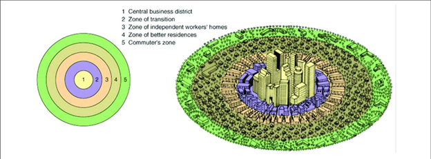
The first zone, called the transition zone, is a mixture of residential buildings and commercial businesses with higher crime rates, poverty, and immigration. The working zone encompasses primarily blue-collar workers. Less educated residents live in this zone, and the jobs matching their skills do not require higher education. However, they can still pursue higher education levels if they want. The zone of better residences, or the educated residential zone, has more educated people with better living standards. They mostly dwell in larger houses detached from each other. Finally, the last zone, the commuter zone, is where the city’s rich people live. These residents usually work close to the CBD but live far away due to their financial ability to pay the transportation costs and commute daily (Planning Tank, 2020).
Sector Model (Hoyt Model)
The Hoyt model, also known as the sector model, is an urban land-use model that predicts the spatial arrangement of activities in large cities and towns. Developed in 1939, this model describes and forecasts how activities are spread around the central business district (CBD) as the population grows. The key difference between the Hoyt model and earlier models is that Hoyt believed activities do not necessarily form concentric rings but rather organize along sectors. Activities are arranged based on their function or purpose. For instance, areas with good access to railways or rivers tend to remain industrial to take advantage of this accessibility.
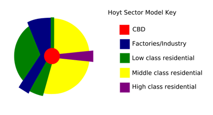
As shown in Figure 3.9, the Hoyt model has five major components. The CBD is the first sector, which is the geographical center of the city and has the highest density, with more skyscrapers than other areas. It is also the oldest part of the city and has many historical and cultural sites. The industrial sector radiates out from the city center and is linked to transportation.
The third, fourth, and fifth sectors are residential areas, divided by socio-economic class. The low-class residential sector consists of high-density areas with poor air ventilation and environmental conditions due to the proximity to factories. People in this sector have shorter work trips. In contrast, the upper and middle-class sectors can afford to live further away from these areas, occupy larger pieces of land, and build suburban-style, detached housing units with better living conditions.
One of the most significant advantages of the Hoyt model is its consideration of the role of transport routes in development. However, it only considers railroads to predict future growth. Also, the model assumes the city is still monocentric, even though in many cases, there is more than one center. Moreover, it does not account for physical features such as rivers or mountains as growth restrictions. (Planning Tank, 2020).
Multiple Nuclei Model
According to the model proposed by C.D. Harris and Edward L. Ullman, an urbanized area has various growth points, around which activities and growth occur. Initially, most cities grow with one center (CBD), but over time, the activities tend to scatter. This leads to the creation of smaller nuclei, attracting people from the surrounding areas. With time, these smaller centers gain importance, grow in size, and affect land use and values. This model is more realistic than previous ones because private cars and sprawling cities have made it impossible to have one center for all economic activities. As a result, this model suits large and expanding cities like New York, Chicago, or San Francisco. Each activity in the area is an independent zone that gradually grows and influences the nuclei in its proximity, as shown in Figure 3.10. These zones are:
- CBD or Downtown area
- Light manufacturing units
- Poor and low-income groups
- Middle-income and working-class groups
- Affluent social groups
- Heavy manufacturing units
- Secondary centers (sub-centers)
- Residential land use in suburbs
- Industrial and manufacturing land use in suburbs
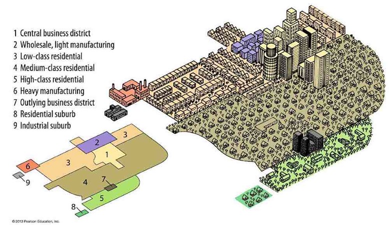
Unlike previous models, this model relaxes the assumption that the land is flat. It presumes that resources and population are evenly distributed throughout the city. While transportation costs play a crucial role in the formation of nuclei, the model assumes that the cost of transportation is uniform and homogeneous across the entire urban area. Similar to agents in previous models, the agents in this model are assumed to be rational, meaning their goal is to maximize utility. Utility is determined by the interplay between transportation costs, labor costs, and rents (bid-rent curve) (Faridi, 2018).
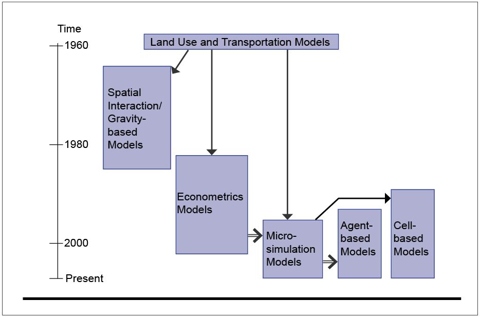
Integrated Land-use Transportation Models
In the preceding section, we observed that early theories and models of land use and urban form lacked consideration of integrated land use and transportation, failing to recognize their mutual impact. While this integration poses a considerable challenge for modelers, given the complexity of modern urban regions, since the 1960s, researchers have made efforts to address these interactions. The crux of these models lies in understanding the relationship between transportation networks, land use, and the location of economic activities, with a central focus on accessibility. Figure 3.11 illustrates the evolution of land-use and transportation models from the 1960s to the present (Van Lierop et al.; Waddell, 2011; Iacono et al., 2008).
The upcoming section will briefly overview different land use transportation interaction models which can be traced back to the 1960s. Lowry (1964) pioneered the development of a model representing the metropolitan area. Lowry’s model, included in the “Spatial Interaction/Gravity-based Models” in Figure 3.3, is recognized as the foundational operational simulation model for urban land-use models.
Gravity Model
In the mid-20th century, the earliest simulation models focusing on the interaction between land use and transportation gained popularity in regional science and quantitative geography. These models, rooted in Newtonian physics and later applied to social physics, were exemplified by the gravity model. Derived from the concept of entropy maximization, the gravity model influenced the development of various spatial interaction models. Unlike more mechanistic approaches, this model, akin to the gravitational concept in physics, establishes a proportional relationship between the number of trips (or interactions) between two zones and the origins and destinations in those zones. Simultaneously, this relationship is inversely linked to the distance between the zones (Wilson, 2021; Iacono et al., 2008). The formula expressing this relationship is as follows:

- Tij is the interaction (or number of trips) between each pair of zones;
- Oi refers to origins at zone i;
- Dj is number of destinations to zone j;
- Ai and Bj are calibration factors that serve as multipliers for balancing total number of trips.
Certainly, the Lowry model (discussed in Chapter 6) stands out as one of the most renowned land use/transportation models utilizing the gravity model. Originating in Pittsburgh, Pennsylvania, this model was crafted to analyze residential and service location patterns. Initially motivated by the need to simulate the impacts of urban renewal and slum clearance on activity distribution within the region, the model, akin to economic theory, categorized industries into basic and non-basic.
In the model, basic industries are those predominantly exporting their products outside the region, while non-basic industries cater to local households and other regional industries. A key assumption of the model is that population distribution aligns with the location of basic industries. In other words, the model posits that first, a basic industry establishes itself in the area (considered fixed and endogenous), and subsequently, the population (workforce) selects their residential location.
The formula representing the location choice based on basic industry incorporates two key assumptions:
- (1) Workers are inclined toward living closer to their workplace, and
- (2) One worker within each household.

Where:
- f(tij) is an impedance function value that refers to the probability of working in zone i and living in zone j;
- tij measures the cost or (dis)utility of movement between zone i and zone j that can be measured by travel time or cost;
- β represents the marginal disutility per unit of time.
Next, using this likelihood, the total number of workers in each zone can be calculated as:
where ei is the employment in zone i, Wj simply measures the relative attractiveness of a zone based on the available land for residential purposes.
The model employs a similar process for non-basic industries to achieve comprehensive coverage. Initially, fixed locations for non-basic industries catering to households and other industries are determined. Subsequently, leveraging the outputs from these initial determinations, a conventional trip-based travel forecasting model is applied. This model calculates network flows in terms of Vehicle Miles Traveled (VMT) by link, providing valuable data to update travel times. Consistent with the iterative nature of most land-use/transportation models, this model repeats the process, continually refining travel times and recalculating the allocation of households and the non-basic employment sector (Iacono et al., 2008).
Simulation Models
Simulation models are essentially activities designed to analyze the impacts of various predicted conditions by expressing the operational components of a system and their interrelationships. To put it simply, any mathematical model requiring extensive computational resources falls under the umbrella of simulation models (Batty, 1976, p.294). These models become necessary when straightforward linear algebraic formulations fall short in addressing the complexities of the situations we aim to understand or predict. The primary objective of simulation models is to predict system behaviors under intricate conditions.
In the context of land-use planning, spatial simulations utilizing dynamic models like cellular automata prove to be valuable tools. In this model, an urban area’s land use is represented by a grid network of cells, with each cell treated as a discrete entity. Cellular automata, with their bottom-up approach, have gained prominence by emphasizing that global and large-scale changes emerge from the interactions of local forces and rules. These models capture spatiotemporal changes across different categories and forecast intricate patterns in land development.
Cellular automata, particularly in recent years, have attracted considerable attention due to their ability to incorporate a range of biophysical and socioeconomic factors. By considering these factors, Cellular Automata models can effectively recognize and predict the dynamics and development of land use (Liao et al., 2016). Agent and activity-based models or cell-based models of urban land use and transportation could now model the changes in a bottom-up format that tried to capture individual behaviors of agents associated with other agents in time and space. While the boldest feature of these models is their level of disaggregate analysis, they can be practical tools for modeling systems that are dynamic and complex, just like urban land use and transportation interactions (Iacono et al., 2008).
Econometric Approaches
Gravity models face a significant limitation in that they are highly aggregated, lacking the ability to capture individual behaviors within the model. The introduction of random utility theory, aimed at understanding decision-making between discrete alternatives, provided researchers with the impetus to explore land-use transportation interactions in a more detailed and disaggregated manner. This theory, centered on individual choices, became instrumental in modeling the interrelated decisions related to location and travel behavior.
As a result, these more detailed model types gained traction alongside simulation models. Econometric models, a category encompassing regional economic models and land market models, emerged as a key avenue for researchers (Iacono et al., 2008). The regional economic input-output analysis provides a highly disaggregate format of the flow and interactions between industries, enabling modelers to incorporate the interactions in a detailed and disaggregate format into land use/transportation forecasts. The work of Leontief first introduced input-output modeling between economic sectors and industries. His model illustrated the flow of goods in an economy. In an economic system, we classify several industries into industrial sectors, each utilizing input from itself and other sectors. The Leontief model assumes that a single sector only serves a particular product and that no products are produced jointly by different sectors. Also, the output quantity solely determines the input quantity (Pan & Richardson, 2015).
Technological advancements, particularly in data storage and computational capacity, coupled with the development of new mathematical and statistical theories like chaos theory (as discussed in chapter 2), have empowered researchers to address many limitations inherent in previous models. These advancements have opened up new possibilities for more refined and accurate modeling of land-use transportation interactions.
Tables 3.3 and 3.44 summarize different econometric and microsimulation models and their specific features.
| Model | Reference | Distinguishing Features |
|---|---|---|
| ILUTE | Salvani and Miller (2005) | Comprehensive urban system microsimulation model; structured to accurately capture temporal elements urban change; activity-travel model includes household member interactions; disequilibrium modeling framework |
| ILUMASS | Moeckel et al. (2003); Strauch et al. (2003) | Descendent of IRPUD model; incorporates microscopic dynamic simulation model of traffic flows and goods movement model; designed with environmental evaluation submodel; |
| Ramblas UrbanSim | Veldhuisen et al. (2000) Waddell et al. (2003) | Entirely rule-based model framework; designed to simulate very large populations Land use model incorporating microsimulations of demographic processes land use development; parcel-level land use representation; high level of household type disaggregation; open-source software developed for general use |
| Model | Reference | Distinguishing Features |
|---|---|---|
| CATLAS | Anas (1982) | Improved representation of economic agents and decision making; explicit treatment of housing markets; economic analysis capabilities |
| MEPLAN | Echenique et al. (1969); Echenique et al. (1990) | Incorporation of spatial input-output model with economic evaluation component; able to forecast commercial trip generation; travel treated as a derived demand |
| TRANUS | de la Barra (1989) | Development supply model simulates choices of developers; sophisticated travel model with combined mode-route choice |
| MUSSA | Martinez (1992) | Incorporation of bid-rent framework for land, floor space markets; detailed representation of transit network in travel model; high level of household type disaggregation |
| METROSIM | Anas and Arnott (1994) | Model extended to commercial real estate markets; addition of dynamic CHPMM housing market model |
| NYMTC-LUM | Anas (1998) | Endogenous determination of housing prices, floor space rents, and wages; high level of spatial disaggregation suitable for transit and land use policy evaluation |
| DELTA | Simmonds (1999) | Microsimulation of demographic changes; treatment of quality in the market for space |
| PECAS | Hunt and Abraham (2005) | Regional econometric model with microsimulation of land development at the parcel level; ability to couple with an activity-based travel model and to apply at supra-regional level |
CONCLUSION
This chapter highlights the crucial need to account for the reciprocal impacts of changes in land use and transportation within urban models. Drawing inspiration from theories and models in economics, geography, and physics, the effort centers around key concepts like accessibility and spatial interaction. While these models simplify the intricate and dynamic urban reality, they provide transportation planners with significant benefits, including a framework by which the future of urban landscape can be forecasted. These forecasts can show how much activity is going to be loaded in specific parts of the city as a result of the improvement in transportation. Or the models help us estimate traffic volume and demand because of induced or added activities.
Over the past few decades, various land-use/transportation models with distinct features and modeling approaches have emerged. With the increase in computer power, digital data, and modeling techniques, a common practice today is to shift from aggregate models, where zones are units of analysis, to disaggregate models that dynamically simulate the behavior of individuals and agents.
The intricate relationships among different forces and agents in disaggregate models can be captured and predicted with the use of large resolution datasets. Policy analysis and decision-making, as described in Chapter 2, are essential objectives in transportation planning, considering various perspectives such as equity and climate change. In this regard, land use and transportation models serve as vital tools for evaluating the performance of our urban and regional transportation systems. Subsequent chapters in this book delve into some of the most recognized models frequently used in transportation planning, starting with basic models, and progressing to detailed transportation planning tools and packages.
Glossary
- Concentric zones is one of the earliest theoretical models that explain the urban structure and formation of social relations, created by Ernest Burgess in 1925
sector or theory of axial development is urban structure theory which states that growth take place around transportation corridors (like highways or rivers) usually originating from urban core. - Agricultural land rent theory is one of the first models that attempts to explain the location of various land uses with respect to costs of transporting goods to the market and land rents, developed by Von Thünen in 1826.
- Trip generation is the first step of four-step travel demand model that predicts number of trips originated from and destinated to various zones within a city.
- Mode choice or modal split is the third step of four-step travel demand model that predicts the means of trips or ratio of trips by each mode from total trips between two zones.
- Urban density is a measure of amount of population, activities or buildings in the unit of space.
- Multi-modal transport system is a transportation system that includes different planned modes such as public transport, walking and biking.
- Polycentric urban forms is more dispersed urban form where multiple independent centers or sub-centers each of which have usually higher density in terms of buildings, and employment from their surroundings.
- Containerization is a new way of transporting goods that uses intermodal containers known as shipping container for moving various types of goods more easily and efficiently.
- Traffic analysis zone (TAZ) is a geographic unit usually used in transportation planning studies which can be bigger or smaller than a block group or even a tract.
- Comprehensive planning is traditional planning method that attempts to establish guidelines for future growth of community via developing goals, vision, programs, plans and missions.
smart growth is a type of development that promotes environmental-friendly, economic viability, and sustainability for future urban developments. - Transit-oriented development is type of development that offers residential, business and leisure activities with a walking range from a public transit station, developed by Peter Calthorpe.
- Peak demand refers to a period of time when the travel demand is at maximum.
- Cost-benefit analysis is a systematic analysis of costs and benefits of projects or alternatives.
- Monocentric city is a urban form in which a core (CBD) accommodates most of business activities and works commute from outer locations to this core.
- Central place theory is an urban geographic theory that attempts to explain the formation of business activities and their services areas in a human settlement, introduced in 1933.
- Input-output analysis also known as (IO) is a modeling technique that disaggregates the economic activities into interactions (demand and productions) between different sectors.
- Economic equilibrium condition refers to a condition or state that demand and supply intersect (equalize) and economic forces are balanced and remain unchanged assuming no external factors.
- Spatial modeling is an instrument for conducting geospatial analyses.
- Radial expansion is a type of land development that is usually take place according to corridors that originate from urban core and extend radially to outer edge of city.
- Marginalized groups are groups or communities that experience discrimination or disadvantage, or exclusion in receiving services.
- Socio-economic mobility refers to movement of people among different social or economic class, which can be either upward or downward.
- Basic industries are the ones that export most of their products outside the region
- Non-basic industries are the industries that serve households and other industries inside the region
- Impedance function is a function that convert travel costs (usually time or distance) to the level of difficulty of getting from one location to the other.
- Bottom-up approach is a participative approach in planning and decision making that plans are usually developed locally and at lower levels and citizens can get involved in the planning process.
- Random utility theory is an econometric theory that states individuals choices are random and can happen differently if the same choice is to be made by a person at different incidents (such as choosing a food from a menu).
Key Takeaways
Key Takeaways
In this chapter, we covered:
- The key theoretical backbone of land use/transportation modeling by which it can be explained why we should integrate land use and transportation.
- Physical systems, agents, and spatial dynamics are the three main components of integrated land use/transportation modeling.
- The earliest attempts to model land-use and transportation modeling, their applications, and their shortcomings.
- Various approaches for contemporary land-use transportation modeling with respect to new computational capacities.
Prep/quiz/assessments
- How is the relationship between land use and transportation shaped? What are the different components within this relationship, and why is it considered a loop?
- How is accessibility formulated in transportation planning, and what factors help measure accessibility?
- What are the main criteria for evaluating land use and transportation plans?
- What are the similarities and differences between Von Thunen’s Monocentric City, Concentric Zones, Hoyt’s Sector, and Multi Nuclei models?
- What are gravity models in land use and transportation planning, and how are they incorporated into land-use transportation models?
References
admin. (2020, September 18). Concentric zone model by Ernest Burgess | Burgess model. Settlement Geography https://planningtank.com/settlement-geography/concentric-zone-model-burgess-model.
Anjomani, A. (2009). Integrated Land Use Transportation Modeling Needs and Legislative Mandates. WSEAS Transactions on Environment and Development https://www.researchgate.net/publication/237474366_Integrated_Land_Use_Transportation_Modeling_Needs_and_Legislative_Mandates
Boarnet, M. G., Hong, A., & Santiago-Bartolomei, R. (2017). Urban spatial structure, employment subcenters, and freight travel. Journal of Transport Geography, 60, 267–276. https://doi.org/10.1016/j.jtrangeo.2017.03.007
Cervero, R., & Wu, K-L. (1997). Polycentrism, commuting, and residential location in the San Francisco Bay Area. Environment and Planning A: Economy and Space, 29(5), 865–886. https://doi.org/10.1068/a290865
Davidson, K. B. (1977). Accessibility in transport/land-use modelling and assessment. Environment and Planning A, 9(12), 1401–16. https://doi.org/10.1068/a091401
Giuliano, Genevieve. 2004. “Land use impacts of transportation investments.” The Geography of Urban Transportation 3: 237–73.
Guiliano, G. (2004). Land Use Impacts of Transportation Investments – Highway and Transit. The Geography of Urban Transportation 3: 237–73. https://trid.trb.org/view/756066
Giuliano, G., & Small, K. A. (1991). Subcenters in the Los Angeles region. Regional Science and Urban Economics, 21(2), 163–182. https://doi.org/10.1016/0166-0462(91)90032-I
Hansen, W. (1959). How accessibility shapes land use. Journal of the American Institute of Planners, 25(2), 73–76. https://doi.org/10.1080/01944365908978307
Hensher, D. A. (2004). Handbook of Transport Geography and Spatial Systems. Emerald Group Publishing Limited eBooks. Emerald (MCB UP). https://doi.org/10.1108/9781615832538
Iacono, M., Levinson, D., El-Geneidy, A., Wasfi, R., & Zhu, S. (2008). Access to Destinations: Monitoring Land Use Activity Changes in the Twin Cities Metropolitan Region. Minnesota Department of Transportation Conservancy.umn.edu. https://conservancy.umn.edu/handle/11299/151332
Liao, J., Tang, L., Shao, G., Su, X., Chen, D., and Xu, T. (2016). Incorporation of extended neighborhood mechanisms and its impact on urban land-use cellular automata simulations. Environmental Modelling & Software, 75, 163–75.
Mandich, M. J. (2019). Ancient city, universal growth? Exploring urban expansion and economic development on Rome’s Eastern periphery. Frontiers in Digital Humanities, 6. https://doi.org/10.3389/fdigh.2019.00018
Meyer, M. D., Institute Of Transportation Engineers. (2016). Transportation planning handbook. Institute Of Transportation Engineers. Wiley.https://users.pfw.edu/sahap/CE450%20Transport%20Policy%20and%20Planning/1.%20Lectures/Books,%20references,%20readings/Transportation%20Planning%20Handbook%20Forth%20Edition.pdf
Miller, E. J., & Soberman, R. M. (2003). Travel demand and urban form. Www.osti.gov. https://www.osti.gov/etdeweb/biblio/20415026
Mohsin, M., & Anwar, M.M. (2015). Identification of land uses through the application of Multiple Nuclei Model in Bahawalpur City, Pakistan: Planning perspectives. Sindh University Research Journal-SURJ (Science Series), 47(3).
Faridi, R. (2018, October 31). Multiple nuclei model of Harris and Ullman. Rashid’s Blog: An Educational Portal. https://rashidfaridi.com/2018/10/31/multiple-nuclei-model-of-harris-and-ullman
Pavlovic, M., Ilic, S., Antonic, N., & Culibrk, D. (2022). Monitoring the impact of large transport infrastructure on land use and environment using deep learning and Satellite Imagery. Remote Sensing, 14(10), 2494. https://doi.org/10.3390/rs14102494
Niedzielski, M. A., & Kucharski, R. (2019). Impact of commuting, time budgets, and activity durations on modal disparity in accessibility to supermarkets. Transportation Research Part D: Transport and Environment, 75, 106–120. https://doi.org/10.1016/j.trd.2019.08.021
Owota, k. M., & michael-olomu, (2023). Ecological zones and socio-economic development in Yenagoa city of Bayelsa state, Nigeria. Wilberforce Journal of the Social Sciences (WJSS) 8(1), 110-127, 10.36108/wjss/2202.80.0160
Rivas, M. E., Suárez-Alemán, A., & Serebrisky, T. (2019). Políticas de transporte urbano en América Latina y el Caribe: dónde estamos, cómo llegamos aquí y hacia dónde vamos. Inter-American Development Bank.
Rodrigue, J. (2020). The Geography of Transport Systems. Routledge.
Sharma, S., Sharma, A., & Kumar, A. (2011). New city model to reduce demand for transportation. Procedia Engineering, 21, 1078–1087. https://doi.org/10.1016/j.proeng.2011.11.2114
Sinclair, R. (1967). Von Thunen and urban sprawl. Annals of the Association of American Geographers, 57(1), 72–87. https://www.jstor.org/stable/2561848
Small, K. A., Verhoef, E.T., & Lindsey, R. (2007). The Economics of urban transportation. Routledge.
Travel Forecasting Resource. (n.d.). Accessed May 12, 2022. https://tfresource.org.
Van Lierop, D., Boisjoly, G., Grisé, E., & El-Geneidy, A. (2017). Evolution in land use and transportation research. Planning Knowledge and Research, 110–131. https://doi.org/10.4324/9781315308715-8
Von Thünen, J.H. (1826). Von Thünen’s Isolated State
Waddell, P. (2011). Integrated land use and transportation planning and modelling: Addressing challenges in research and practice. Transport Reviews, 31(2), 209–229. https://doi.org/10.1080/01441647.2010.525671
Wegener, M. (2004), “Overview of Land Use Transport Models”, In Hensher, D.A., Button, K.J., Haynes, K.E. and Stopher, P.R. (Ed.) Handbook of Transport Geography and Spatial Systems (, Vol. 5), Emerald Group Publishing Limited, Bingley, pp. 127-146.
J. Barkley Rosser. (2021). Entropy and complexity in urban and regional systems. In Reggiani, A., Schintler, L. A., Czamanski, D., & Patuelli, R. (Eds.). (2021). Handbook on Entropy, Complexity and Spatial Dynamics: A Rebirth of Theory?. Edward Elgar Publishing.
Zhang, L., Xu, W., & Li, M. (2009). Co-Evolution of Transportation and Land Use: Modeling Historical Dependencies in Land Use and Decision-Making. OTREC-09-07. Portland, OR: Transportation Research and Education Center (TREC), 2009 https://doi.org/10.15760/trec.96
Zhou, Z., Yang, Z., Zhang, Y., Huang, Y., Chen, H., & Yu, Z. (2022). A comprehensive study of speed prediction in transportation system: From vehicle to traffic. iScience, 25(3), 103909. https://doi.org/10.1016/j.isci.2022.103909
Concentric zones is one of the earliest theoretical models that explain the urban structure and formation of social relations, created by Ernest Burgess in 1925
sector or theory of axial development is urban structure theory which states that growth take place around transportation corridors (like highways or rivers) usually originating from urban core.
Agricultural land rent theory is one of the first models that attempts to explain the location of various land uses with respect to costs of transporting goods to the market and land rents, developed by Von Thünen in 1826.
Trip generation is the first step of four-step travel demand model that predicts number of trips originated from and destinated to various zones within a city.
Mode choice or modal split is the third step of four-step travel demand model that predicts the means of trips or ratio of trips by each mode from total trips between two zones.
Transportation network is a system or graph of corridors distributed in space that permits movement of people and goods.
Traffic analysis zone (TAZ) is a geographic unit usually used in transportation planning studies which can be bigger or smaller than a block group or even a tract.
Comprehensive planning is traditional planning method that attempts to establish guidelines for future growth of community via developing goals, vision, programs, plans and missions.
smart growth is a type of development that promotes environmental-friendly, economic viability, and sustainability for future urban developments.
Transit-oriented development is type of development that offers residential, business and leisure activities with a walking range from a public transit station, developed by Peter Calthorpe.
Peak demand refers to a period of time when the travel demand is at maximum.
Input-output analysis also known as (IO) is a modeling technique that disaggregates the economic activities into interactions (demand and productions) between different sectors
Economic equilibrium condition refers to a condition or state that demand and supply intersect (equalize) and economic forces are balanced and remain unchanged assuming no external factors.
Spatial modeling is an instrument for conducting geospatial analyses.
Radial expansion is a type of land development that is usually take place according to corridors that originate from urban core and extend radially to outer edge of city.
Socio-economic mobility refers to movement of people among different social or economic class, which can be either upward or downward.
• Basic industries are the ones that export most of their products outside the region
Non-basic industries are the industries that serve households and other industries inside the region
Bottom-up approach is a participative approach in planning and decision making that plans are usually developed locally and at lower levels and citizens can get involved in the planning process.
Refer to changes that take places into dimension both in space and time.
