6 Land-Use and Transportation Modeling II: Lowry Model
Chapter Overview
Chapter 6 delves into the Lowry model, a widely utilized integrated land-use and transportation model. It explores the fundamentals of the Lowry model, which aids in forecasting the activity locations of residential, basic, and non-basic economic sectors in urban areas. By presenting the model’s assumptions, equations, and application steps, this chapter aims to equip students with the necessary knowledge for applying Lowry-type models. The Lowry model is one the most famous and inspirational landuse/transportation models and its framework has been adopted by many modelers. This chapter attempts to explain how gravity-based models can be used as spatial allocation models for different types of activities. The final section of the chapter examines the matrix formation of the Lowry model as a mathematical solution. Additionally, it briefly introduces three extensions of Lowry-type models, including the Lowry-Garin Model, the Projective Land Use Model (PLUM), and the Time-Oriented Metropolitan Model (TOMM).
Learning Objectives
- Explain the framework of Lowry-type models and relate its most essential components to transportation planning goals.
- Explain the process of using gravity-based models as spatial allocation models in Lowry type models.
- Summarize essential steps for building the Lowry model and recognize and categorize the required data for building the model.
- Summarize essential steps for building the Lowry model and recognize and categorize the required data for building the model.
Introduction
As highlighted in earlier chapters, spatial models play a crucial role in addressing the goal of forecasting and projecting future land use change. Back in 1960, when capacities for large-scale computation increased, modelers started to develop aggregate and zonal-based models to describe and simulate land use and transportation activities at a granular level (TAZ, blocks, block groups, etc.) (Iacono, Levinson, & El-Geneidy, 2008; Wegener, 1995). The outcomes of these models can point out where activities or transportation potentially occur in future. The end product of these models are usually amount of change in terms of land use (population and employment growth by spatial units of the models. The subject of this chapter, the Lowry Model, is a prototype of this era, developed by Ira Lowry as part of a regional economic study of the Pittsburgh metropolitan region rather than as a land-use transportation study, however, its simplicity and ease of implementation widely inspired land use modeling (Boyce and Williams 2015).
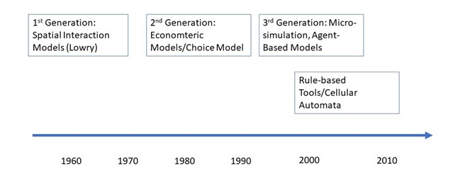
Spatial models are utilized for forecasting land use changes using a zonal system. Following the projection of future land uses, regional employment and income distribution information is used to allocate the labor force across different economic sectors and zones. It’s worth noting that these groups model assume linear relationship and homogeneity, all of which may affect the accuracy and reliability of the results (Hensher, 2004). Figure 6.1 depicts the timeline for the evolution of land use models. As the figure shows, the first generation of models, relying on spatial interactions or gravitational forces has started with Lowry type models
Lowry model
The Lowry model, developed by Ira Lowry for the Pittsburgh metropolitan region in the 1960s, was one of the first land-use-transportation models that incorporated both generation and allocation of activities within its structure. Two significant components of the model are (1) an economic base mechanism and (2) a gravity model as a function of the attractiveness between activities. The spatial dimension of the model is a matrix computed from two major types of trips: home-to-work and home-to-shop journey trips. One of the strengths of the Lowry model is its high applicability and modest need for data (Jun & Moore, 2002).
However, there are some limitations of Lowry-type models. These models lack an underlying economic or behavioral theory (Berechman & Small, 1988). Also, the model leans towards the economy’s demand side, ignores other factors such as supply, and considers highly aggregated economic sector data (basic vs. non basic), which are the frequently mentioned drawbacks of the Lowry model.
Additionally, the limitation that it is demand-driven means it tends to underestimate the supply of land as it mainly responds to increases in basic employment. Furthermore, the model disregards the role of policies and decisions made by policymakers which have implications on land use and transportation. Another limitation is that it does not consider transportation systems and technologies that impact urban development. Figure 6.2 shows how the Pittsburg metropolitan region was divided into a set of one square mile grids for the modeling needs.

6.3.1 Lowry Model Framework
The Lowry Model operates as a heuristic model where the distribution of basic employment determines how land is allocated for residential and retail sectors. This model distinguishes between two employment sectors: basic and retail (non-basic). The retail sector encompasses activities meeting local population needs, such as local market areas, services, shopping centers, local government, schools, and office buildings. On the other hand, basic employment includes site-oriented economic activities, with the assumption that the location of industrial activities (basic sector) is independent of residential and retail activities. In other words, the choice of location of business firms is indifferent to the size and location of residential areas (Lowry, 1964).
A critical assumption of the model is that industry, the basic sector, drives regional growth (or decline), and the basic employment in each zone of the urban area is exogenously determined (i.e., outside the model). This means that the distribution of employment across zones is an input to the model, along with travel time across zones. Industry (basic sector) drives the demand for labor, impacting total population change in the area. The population’s demand for services and goods influences changes in the non-basic sector, which further affects the demand for labor. According to this logic, based on the employment distribution in the basic sector, the model projects population change and the residential location of employees in urban areas (zones) using a work-to-residence distribution function. The locational distribution of residents serves as the basis for distributing retail employment, determined by a resident-to-shop distribution function. This iterative process continues until an equilibrium state is achieved, as land allocation to the retail sector creates employment opportunities, leading to the need for additional residential areas and new round of retail activities, and so on.
The Lowry Model also assumes that agents’ location choice decisions, shaped mainly by employment accessibility, influence land-use patterns over time in metropolitan areas. In addition to location choice, distribution functions and attractiveness are integral components of the Lowry Model framework. Zones can be any unit of geographical aggregation like census tracts, census block groups, or traffic analysis zones. A zone’s relative attractiveness can be calculated via the gravity concept (Hansen, 1959) and its mathematical formula widely used across many disciplines. In the Lowry model, the factor used to derive the relative attractiveness of each zone is accessibility (the distance from each zone to retail land uses and employment).
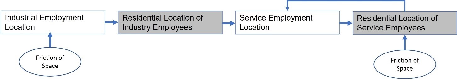
Figure 6.3 illustrates how two gravity models, one for residential and the other one for retail services, work together through an iterative process to determine the land-use pattern for the study area. The term “export” industry in this figure represents the same basic industry we identified above. This is because it is believed that the basic industry is an export-based industry and will not be affected by the existing conditions in the region, thus exogenous to the model.
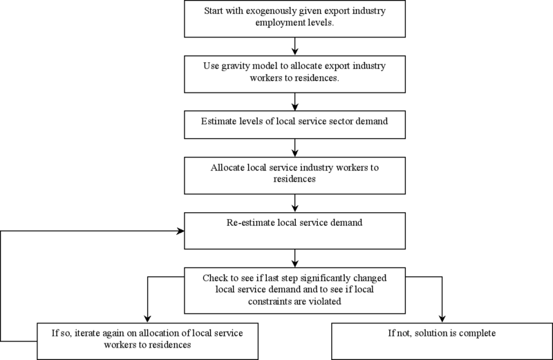
According to Figure 6.3, the interaction between each pair of zones positively depends on the concentration of activities. It negatively depends on the friction factor between the zones which commonly is travel distance or cost (Acheampong & Silva, 2015). Figure 6.4 shows the general steps and procedures for forecasting future land uses based on the three sectors (basic employment, retail employment, and residential locations).
Lowry model basics and equations
In the preceding section, we introduced the Lowry Model and its framework. This section explains the process of constructing this model within a defined geographical study area, accompanied by the relevant mathematical methods and formulas.
After deriving population and service employment from basic employment data, the subsequent step involves allocating these activities to spatial locations or zones within the urban region. Each zone is subject to various land allocation constraints, considering both residential and retail activities. These constraints are integral to the model, ensuring, for example, that the population in each zone adheres to a specified density threshold. Similarly, the model imposes a minimum size constraint for the service sector, ensuring that no retail center is assigned to a zone unless it meets specified minimum market requirements (Jun & Moore, 2002).
Once the population and activities are calculated and land is allocated to each zone, it becomes crucial to assess whether the computed distributions align with the input data. This verification process is accomplished by iteratively feeding back the forecasted population and employment back into the model, aiming to align the forecasted results with the observed ones. The next section outlines the mathematical formulas and essential steps guiding the process from inception to completion in building the model, but first, all the factors and data needed for this modeling framework are listed below:
Model Inputs: exogenous data:
- Total land
- Unused land
- Basic employment: industry or basic sector’s jobs allocated to zones.
- Transportation network (travel time).
- Friction factor between zones.
- Ratios of:
- Total population to workers
- Retail/service (non-basic sector) workers to population.
- Zones’ constraints (e.g., population density limits, minimum market requirements)
Model Estimates
• Residential Estimation:
- Land available for housing
- Total population
- Population distribution (subject to constraints)
• Retail Sector Estimation:
- Retail employment
- Distribution of retail employment (subject to constraints)
- Retail land use
- Subject to land availability
Thus, the output of the model would be the projection of residential activity(population) and service and basic employment rate for each spatial unit of analysis.
Lowry Model equations
As outlined above, the model’s exogenous input includes data for total land area, unused land area, land designated for basic activities by area, basic employment, and transport network characteristics for the travel impedance function. Additionally, the constraints integrated into this model include:
- the quantity of land available for development,
- the population density threshold regulated by local government, and
- c) the minimum threshold for the economic justification of service businesses, categorized as neighborhood, local, or district, and metropolitan (Briassoulis, 2020).
Once all this information is gathered, the model is applied to the study area in two main steps, involving two sets of calculations.
- The first step estimates the population’s location based on total employment, and
- the second step estimates the total service employment based on the the results from Step 1.
Following the completion of these two steps, the model checks for consistency between the predicted distribution of the population and the distribution used to compute potentials, ensuring they align. If inconsistencies arise, the model iteratively repeats the same procedure until equilibrium is achieved. After finishing the two steps, the model checks for consistency between the predicted distribution of the population and the distribution used to compute potentials to find out if they coincide. If they do not, the model repeats the same procedure iteratively.
In the first step, the model must compute the urban region’s population based on basic employment data. In general, total employment (E) in an area is the sum of basic and service sectors employment:

Where
B is basic employment
S is service employment
For the first set of calculations, we will proceed with total population estimation according to basic sector employment and retail sector employment magnitude based on the calculated population. For this task, we could use the following formulas:
- We assume that the total population (P) depends on basic sector employment. Thus, P can be calculated as follows:

Where
f is a ratio representing persons per employee in the basic sector
- Another main assumption in the Lowry model is that employment of Kth retail sector is proportional to the population according to:

Where
 is a ratio representing the employment per person living in the area
Solving the presented equations gives us the magnitude of total employment, population, and retail employment. The following formulas are also applicable for these calculations.


After calculating the magnitude of total employment, population, and retail employment, the next step includes deriving the amount of land available for residential use in each zone (j) that is represented by:

Where
 is the total land in zone j
 is the total unused land in zone j
 is the total land for basic industries in zone j
 is the total land for retail sector in zone j
After identifying the total land available in each zone and providing the estimate of the total population and employment for each sector, we can calculate the allocation of activities to each zone of the study area. We can achieve this by applying a gravity model which considers the travel impedances function as the travel costs between each pair of zones. The mentioned gravity model is as follows:
Where:

the i subscript refers to all the destinations for work commutes (employment), and f1(cij) is the cost attribute associated with the trip from origin zone (residential) to destination (employment).
We must apply a constraint when allocating the population to different zones to find whether there is a maximum population density constraint violation. The condition check can be verified using the following formula:

Where:
zH is the population density for zone j
Similarly, for the allocation of total employment in retail sector k, EK is assumed to be determined according to the total population. Another gravity model is needed to allocate retail employment using a travel impedance function, which is a function of generalized travel cost for the retail sector:
Where:

gk and qk are the parameters or coefficients that are determined empirically and refers to the importance of population and employment in the market. These values should be calculated manually because they can vary for different case studies.
f2(cij) is the generalized travel cost function for the retail sector.
Another important constraint is limiting the dispersion of retail employment. In fact, this constraint imposes a minimum-size constraint (zk) according to the magnitude of employment in sector k in zone j. This constraint prevents the model from allocating retail establishment in zone j if the minimum size needed to justify this activity is unmet. The mathematical formula for this constraint is as follows:

Next, the third constraint is applied to the model to ensure the amount of land allocated for retail establishments does not exceed the amount available. In other words, this constraint does not allow the model to allocate a negative amount of land for residential purposes. The mathematical format for this constraint is:

Finally, calculating the population for each tract or zone and the number of employments in basic and service (retail section), residential, basic, and retail land use for each zone should be derived using land conversion ratios for each of the three sectors. It is important to pay attention to the constraints for population density and land allocated to the retail section for each zone. The simple formula for this step is:

Where
e1 is ep, eB or eR
X1i is Pi or EBi or ERi
Since the Lowry model includes several equations, variables, factors, and parameters, it would be beneficial to review these values again to avoid confusion. In the following, all variables and parameters used in the Lowry model are listed:
| Variables | Superscripts and Subscripts |
|---|---|
| A= area of land (thousands of square feet) | U= unusable land |
| E=employment (number of persons) | B= basic sector |
| N=population(number of households) | R= retail sector |
| T=index of trip distribution | H= household sector |
| Z=constraints | k = class of establishments within retail |
| sector (k=1,…,m) | |
| i,j = tracts or zones within region (i,j=1,…,n) | |
| a, b, c, d, e, f, g = coefficients |
Additionally, the two most important and principal equations of the Lowry model, by which the number of households or population and demand and distribution of retail employment for each zone can be calculated, are worth mentioning again:

Where Nj is the households located to tract j,
Ei is the total employment at tract I, that refers to the basic employment at the base year (the retail employment is calculated according to households information and will be added to the total employment in next iterations).
Tij is trip distribution index from tract i to tract j.
And,
![E_j^k=b^k[\sum_{i}{\frac{c^kN_i}{T_{ij}^k}+d^kE_j}]](https://uta.pressbooks.pub/app/uploads/quicklatex/quicklatex.com-7a8c68cb8e81b231255efcb24c843a12_l3.png "Rendered by QuickLaTeX.com")
where Ejk is the retail employment for type k establishment at tract j,
Ni is number of households at tract i,
Ej is total employment at tract j,
Tij is trip distribution index for type m shopping trip from tract i to tract j,
bk, ck, and dk are constant coefficients for type m establishment.
The Lowry model’s outputs here are Nj And Ej both of which together depicts the rate of growth or development of each neighborhood in the forecasting year. It should be noted that depending on the categories of employment, E can be further separated to different industries. Thus, the more disaggregate the input, the more accurate would be results in terms of the composition the of activities for each data points (spatial units). For example, after implementing the model, we may forecast number of workers in trade, retail, warehousing, information sector, finance and real estates, and so on.
Brief overview of the model extensions
Numerous models have been built upon the Lowry Model. The Time Oriented Metropolitan Model (TOMM) is one of the first derivations of the Lowry model, developed for the Pittsburg Community Renewal Plan. While this model adopted the basics of the Lowry model, two major additions were applied. First, an incremental (not single-year) approach was introduced, centering on the fact that all forecasted changes do not occur in the forecasting year. This revision thus added the time element into the model. Second, this model divided the population into different socio-economic groups to enhance the model’s explanatory power (Crecine, 1968).
The Projective Land Use Model (PLUM) is another adaptation of the Lowry model that Goldner (1971) developed for the San Francisco Region. The modifications of this model are taking into account differences in zone sizes, the use of an intervening opportunities model to allocate population and employment, disaggregating the model in terms of model parameters according to spatial units, zone-specific activity rates, and population-serving ratios for different services (Goldner, 1971).
The University of Cambridge in the U.K. introduced a British version of the Lowry model that serves urban planning analyses on a town scale. This model is widely applied in several Chilean towns (mainly in the Santiago Metropolitan area) as well as British towns. Using floor space as a measure of location attractions, the advantage of this model is that it incorporates the supply side of the urban land market, which was missing in the original version of the Lowry model. Incorporating floor space as a measure of gravity constrains the demand for space for various activities seeking to locate in different certain zones (Briassoulis, 2020).
The matrix formation of Lowry’s model – Garin (1966)
In this section, we offer a concise overview of the matrix formation of the Lowry model. To address the issue of infinite model iterations, Garin (1966) devised a relatively straightforward yet logical approach for applying the Lowry model.
In this formulation, the residential location of basic employment is calculated by the travel impedance function between each pair of zones (aij) and multiplication by the participation of labor rate in zone j. The formula is:

Where pb is the basic population vector and
A= [aij] = [a’ijaj]
A’= [alij] is the journey to home distribution matrix
Also, [α] is the labor participation rate diagonal matrix.
In a hypothetical area with only three zones the labor participation rate matrix journey to home distribution would look like the following:
| Zone | 1 | 2 | 3 |
|---|---|---|---|
| 1 | 61.3% | 0 | 0 |
| 2 | 0 | 44.1% | 0 |
| 3 | 0 | 0 | 79.8% |
| Zone | 1 | 2 | 3 |
|---|---|---|---|
| 1 | 20 | 28 | 39 |
| 2 | 25 | 18 | 45 |
| 3 | 54 | 46 | 10 |
A similar procedure can be done for the location of population-serving activities but with two differences. First, the home-based journey to shop is used for the travel impedance function, and the β diagonal matrix, which represents the population-serving employment ratio, replaces the α diagonal matrix. This step can be formulated as:
![E^{(1)} = P^b \cdot B = P^b [\beta] B'](https://uta.pressbooks.pub/app/uploads/quicklatex/quicklatex.com-5dcc95e16a30374e5ca1d3d045b2f65c_l3.png "Rendered by QuickLaTeX.com")
Where 1 refers to iteration number, B’= [b’ij] is the journey to shop distribution matrix, and [β] is the population-serving employment ratio, diagonal matrix.
Now if we combine the basic formula for the first and second steps, we have:


This will now generate a new non-basic employment (E(2)).
Where

Applying successive iterations in the same way, additional employment and population are generated (constraints should be taken into account at this point).
As a result, the sum of population and employment is equal to the following two equations, and I is the identity matrix. The formulation of population and employment are as follows:

As a result, the sum of population and employment is equal to the following two equations, and I is the identity matrix. The formulation of population and employment are as follows:

I in this formula denotes the identity matrix.
Under certain conditions on the product matrix AB, the matrix series (between parentheses) converges to the inverse of the matrix (I – AB). Thus, we can write:

and

conclusion
In this chapter, we introduced the first and one of the most famous land use/transportation models, which is based on gravity and spatial interactions approach and econometrics. This model divides the region into small zones and creates a big dataset of the basic industry and then use that information along with friction of space to predict distribution of population and employment. The Lowry model has been proven useful for MPOs and several extensions has been derived based on the principals of these models. All that said, the Lowry model has limitations such as aggregation bias, or ignoring the role of supply along with demand (it is a demand-driven model), or the role of policy agenda and decision making of the region, or role of technological advancement specially in transportation. It is such limitations that have led the modelers to explore newer paradigms and approaches such as discrete choice models or agent- and activity-based models.
Key Takeaways
In this chapter, we covered:
- Different land-use and transportation modeling approaches were dominant through different time periods.
- The theoretical background, modeling framework, and components of the Lowry model
- Strengths and setbacks of the Lowry model
- The history, basics, steps, and procedures of applying the Lowry model
- Data required for building the Lowry model.
- The extensions of the Lowry model and matrix formulation of the model for simplifying model calculations.
Prep/quiz/assessments
- What are the main principles of gravity/spatial interaction models? What are some of the setbacks of these models (Lowry Model)?
- Describe the Lowry model’s exogenous and endogenous data components and explain the various trip purposes considered in this modeling framework.
- Explain the various trip purposes considered in the Lowry modeling framework.
- What are the two most important constraints incorporated in the Lowry model? Why are these constraints embedded in it?
- Name one of the Lowry Model’s extensions and explain it thoroughly.
Glossary
- Spatial models are models that utilize a zonal system by which a study area is disaggregated to smaller units (such as TAZ or tract) usually using GIS-based methods.
- Gravity/Spatial Interaction Type Integrated Models are models that try to estimate or predict spatial interactions between variables among neighborhoods, cities or regions.
- Utility maximization is concept that indicates that agents like organizations or individuals always seek to maximize their level of satisfaction or utility be performing a course of action.
- Demand-driven model is a type of model in which the supply side of land as well as other factors such as policies or programs are ignored and the model predictions are based on the demand component.
- Simulation models are models that are used when the interactions among factors are more complex than a simple linear function and usually high computational capacities are needed for solving the problem.
- Cellular Automata is a model that includes a number (array) cells, and each cell can have a status among K discrete states. As time progresses, cells will adjust their states according to their states as well as states of their nearby neighborhood, a process which is specified by a set of transition rules.
- Heuristic models are usually based on probability and their foundations or structures do not necessarily comply with the theory, resulting in probable behaviors expressed by agents.
- Basic employment refers to those industries whose products are shipped and used by the demand outside of their location such as a mining factory.
- Work-to-residence distribution function is a function of Lowery model that predicts the residential location of the employees in urban areas by the distribution of basic employment.
- Resident-to-shop distribution function is a function in Lowery model that predicts the distribution of retail employment in urban areas by the distribution of residential locations.
- Attractiveness of each zone is a measure for quantifying the gravity of a zone for attracting trips, population, employment, etc.
- Travel impedance function is a function that uses travel time or distance and quantifies how difficult it is to go from one location to another.
- Land conversion ratios is a function that estimates the total amount of land needed for a particular land use type with respect to basic and non-basic employment and residential population.
- Explanatory power is a measure that shows how good the model is fitted to the observed (input) data and how accurate the statistical inferences are accordingly.
- Intervening opportunities model is a model that indicates flow of trips between zones are not totally dependent on distance but rather is related to the accessibility of opportunities that can satisfy the purpose of the trip.
- Diagonal matrix a matrix in which all values except for the values in the main diagonal are zero.
References
Acheampong, R. A., & Silva, E. A. (2015b). Land use–transport interaction modeling: A review of the literature and future research directions. Journal of Transport and Land Use. https://doi.org/10.5198/jtlu.2015.806
Batty, Michael. 1976. Urban modelling: Algorithms calibrations, predictions. Cambridge Urban and Architectural Studies 3. Cambridge ; New York : Cambridge University Press.
Berechman, J. (1988). Modeling land use and transportation: An interpretive review for growh areas. UC Berkeley: University of California Transportation Center https://escholarship.org/uc/item/4nw2t7n5
Briassoulis, Helen. 2020. Analysis of land use change: Theoretical and modeling analysis of land use change: Theoretical and modeling approaches. WVU Research Repository, 2020. https://researchrepository.wvu.edu/cgi/viewcontent.cgi?article=1000&context=rri-web-book
Crecine, John P. 1968. “A dynamic model of urban structure.” Rand Corp Santa Monica CA. https://apps.dtic.mil/sti/pdfs/AD0666655.pdf
Engelen, G., White, R. D., Uljee, I., & Drazan, P. J. (1995). Using cellular automata for integrated modelling of socio-environmental systems. Environmental Monitoring and Assessment, 34(2), 203–214. https://doi.org/10.1007/bf00546036
Goldner, W. (1971). The Lowry Model Heritage. Journal of the American Institute of Planners, 37(2), 100–110. https://doi.org/10.1080/01944367108977364
Hansen, Walter G. 1959. “How Accessibility Shapes Land Use.” Journal of the American Institute of Planners 25 (2): 73–76.https://doi.org/10.1080/01944365908978307
Hensher D. A. (2004). Handbook of transport geography and spatial systems. Elsevier.
Hunt, J. A., & Simmonds, D. C. (1993). Theory and application of an integrated land-use and transport modelling framework. Environment and Planning B: Planning and Design, 20(2), 221–244. https://doi.org/10.1068/b200221
Iacono, M., Levinson, D., & Levinson, D. (2008b). Models of transportation and land sse change: A guide to the territory. Journal of Planning Literature, 22(4), 323–340. https://doi.org/10.1177/0885412207314010
Jun, M., & Moore, J. E. (2002). The Lowry model revisited: Incorporating a multizonal Input-Output model into an urban land use allocation model. Review of Urban & Regional Development Studies, 14(1), 2–17. https://doi.org/10.1111/1467-940x.00045
Levinson, D., Liu, H. , Garrison, W., Danczyk, A. , Corbett, M. , & Dixon, K. . (2014). Fundamentals of Transportation. Wikimedia. https://upload.wikimedia.org/wikipedia/commons/7/79/Fundamentals_of_Transportation.pdf
Lowry, I. S. (1964). A Model of Metropolis. Rand Corp Santa Monica CA. https://www.rand.org/pubs/research_memoranda/RM4035.html
Masser, I., Karpe, H., Ernst, R., & Klatt, H. (1971). Possible applications of the Lowry model. Planning Outlook. https://doi.org/10.1080/00320717108711457
Meyer, Michael D. 2016. Transportation Planning Handbook. 4th Edition. John Wiley & Sons.
Wegener, M. 1995. Current and future land use models. In Land Use Model Conference. Dallas: Texas Transportation Institute (Vol. 2, pp. 119-131).
Spatial models are models that utilize a zonal system by which a study area is disaggregated to smaller units (such as TAZ or tract) usually using GIS-based methods.
Demand-driven model is a type of model in which the supply side of land as well as other factors such as policies or programs are ignored and the model predictions are based on the demand component.
Heuristic models are usually based on probability and their foundations or structures do not necessarily comply with the theory, resulting in probable behaviors expressed by agents.
Basic employment refers to those industries whose products are shipped and used by the demand outside of their location such as a mining factory.
Work-to-residence distribution function is a function of Lowery model that predicts the residential location of the employees in urban areas by the distribution of basic employment.
Resident-to-shop distribution function is a function in Lowery model that predicts the distribution of retail employment in urban areas by the distribution of residential locations.
gravity model is a type of accessibility measurement in which the employment in destination and population in the origin defines thee degree of accessibility between the two zones.
Attractiveness of each zone is a measure for quantifying the gravity of a zone for attracting trips, population, employment, etc.
Travel impedance function is a function that uses travel time or distance and quantifies how difficult it is to go from one location to another.
Land conversion ratios is a function that estimates the total amount of land needed for a particular land use type with respect to basic and non-basic employment and residential population.
Explanatory power is a measure that shows how good the model is fitted to the observed (input) data and how accurate the statistical inferences are accordingly.
Intervening opportunities model is a model that indicates flow of trips between zones are not totally dependent on distance but rather is related to the accessibility of opportunities that can satisfy the purpose of the trip.
Diagonal matrix a matrix in which all values except for the values in the main diagonal are zero.
