Second Step of Four Step Modeling (Trip Distribution)

Qisheng Pan; Soheil Sharifi

11 Second Step of Four Step Modeling (Trip Distribution)

Chapter Overview

This chapter describes the second step, trip distribution, of the four-step travel demand modeling (FSM). This step focuses on the procedure that distributes the trips after trip generation has been modeled, meaning after trips generated from or attracted to each zone in the study area are understood. The input for this step of FSM is the output from the previous step discussed in Chapter 10, trip generation plus the interzonal transportation costs introduced in this chapter. Based on the concepts of the gravity model, the trip flows between pairs of zones can be calculated as an origin-to-destination (O-D) matrix. The essential concepts and techniques, such as growth factors and calibration methods, for this step are also discussed in this chapter.

Learning Objectives

Explain trip distribution and how to relate it to the first step (trip generation) results.
Summarize the factors that determine the level of attractiveness of zones in a travel demand model.
Summarize and compare different methods for trip distribution estimation within FSM.
Complete the trip distribution step by balancing total trip productions and attractions after the trip distribution step.

Introduction

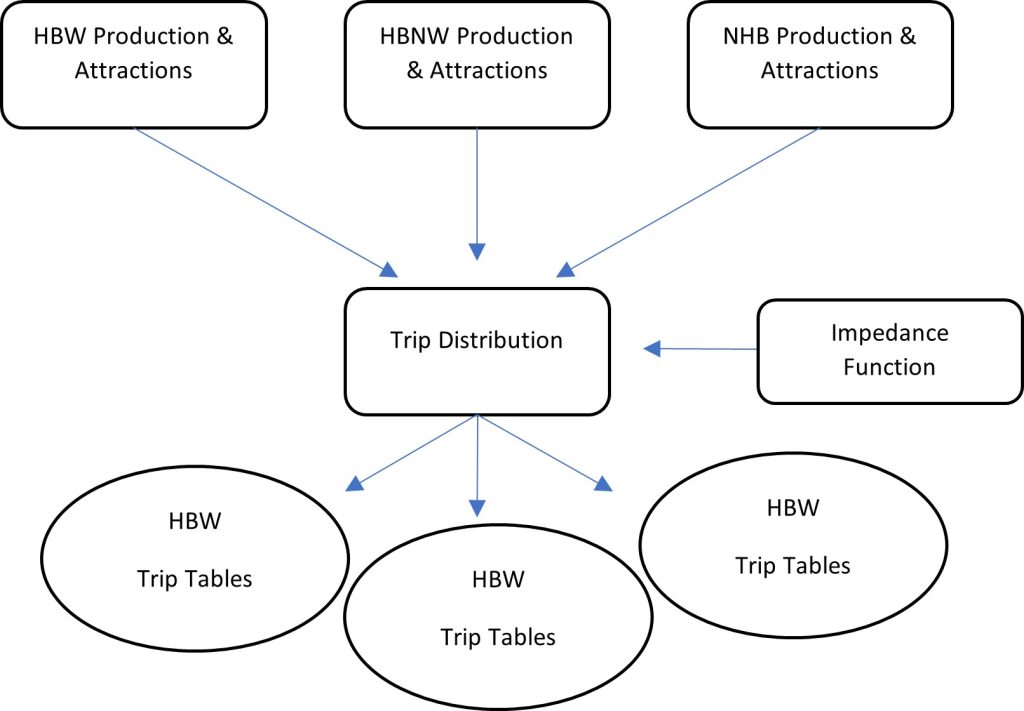
This chapter delves into trip distribution, which is the second step of the Four-Step Model (FSM). After generating trip productions and attractions (P-A trips) by zone in the first step, the next task is to compute the number of trips between each pair of zones, referred to as trip distribution. These outputs are commonly known as Origin-Destination pairs (O-D pairs or Tij, as discussed in Chapter 9), indicating the number of trips between Zone i (origin) and Zone j (destination) (Levine, 2010). Essentially, trip distribution transforms the outcomes of the first FSM step into a comprehensive matrix detailing origins and destinations in Traffic Analysis Zones (TAZs). It also considers travel impedance factors, such as travel time or cost, for each O-D pair. Figure 11.1 illustrates the input (P-A trips) and outputs (trip tables) of this step in the model, highlighting the role of impedance functions initially introduced in Chapter 3 and discussed further in this chapter.

trip attractions and productions resulting in a matrix for each trip purpose. — **Figure 11.1** Trip distribution inputs and outputs From “Introduction to Urban Travel
Demand Forecasting” by NHI In National Highway Administration (Ed.), Introduction to Urban Travel Demand Forecasting. 2005 American University. In the Public domain.

Recall from Chapter 10, that each step of the FSM answers a question specific to the step but central to model determining travel demand in a study area. For the trip distribution step, the main question is “What portion of trips produced in or attracted to a zone would go to each of the other zones?” There are several methods typically used to estimate trip distribution. While growth factor models and the intervening opportunities model are used, the gravity model is the most common.

There are a few foundational components to consider prior to calculating trip distribution. It is important to note that these components are independent of the FSM framework, or the methods used for trip distribution estimation. However, they serve as inputs for estimating trip distribution. As previously mentioned, trip distribution constitutes the second step of the FSM, where trip productions are allocated to all other zones. The outcomes yield a matrix that displays the number of both intrazonal and interzonal trips in a single table (Lincoln MPO, 2011).

The attractiveness of a zone is influenced by several factors (Cesario, 1973):

Uniqueness: This factor indicates how unique a service or employment center is and thus attracts more trips regardless of distance.
Distance: The spatial separation, distance, between two zones plays an impedance role, meaning that the further the two zones are from each other, the fewer trips will be distributed between them.
Closeness to other services: The assumption is that proximity to other desirable services will result in more trips to that zone within an urban area.
Urban or rural area: The assumption is that the attraction rate for a zone differs based on its urban or rural classification, while controlling for other factors.

In addition to the destination’s attractiveness factors, the origin’ has an emissivity factor, which is usually represented by population, employment, or income (Cesario, 1973). With a general understanding of the factors affecting trip distribution from origin and destination, we can now proceed with an introduction to methodology.

Gravity Model

As we discussed, the gravity model is the most common method used to estimate trip distribution. Gravity models are easy to understand and very accurate, and they can also accommodate varied factors such as population, employment, socio-demographics, and transportation systems. Almost all U.S. Departments of Transportation (DOTs) use gravity models. In contrast, the Growth Factor Model, discussed in a subsequent section, requires additional data about trip distribution in the base year and an estimate of the number of future trips in each zone, which is only sometimes available (Meyer, 2016).

It is important to remember that the Gravity Model is built based on the number of trips made between two zones. The number of trips is directly linked to the total number of attractions in the destination zone and inversely proportional to a function of cost, which may be represented by travel time or trip cost (Council, 2006). The formula gets its name from Newton’s Law of Gravity, which states that the attractiveness between two bodies is related to their mass (positive attraction) and the distance between them (negative attraction) (Verlinde, 2011). In transportation modeling, the two main factors are trip production and attraction, along with the time duration of travel or the cost of travel. While using the gravity model is simple, determining the optimal value for the impedance factor can be difficult. This value is highly dependent on the context and can vary by circumstances.

Equation below shows the fundamental equation of trip distribution:

Trips between TAZ1 and TAZ2=Trips prodduced in TAZ1*(Attractiveness of TAZ2 /Attractiveness of all TAZs

As equation (1) shows, the total trips between zones are equal to the products of the trips produced in a zone, a ratio of the attractiveness of the destination zone, and the total attractiveness of all zones. We can represent the gravity model in several different ways. Remodifying equation the original equation, the gravity model can be rewritten as:

Trips_ij=Productions_i*(Attractions_j*FF_ij*k_ij/∑Attractions_j*FF_ij*k_ij)

Where Trips_ij is the number of trips between zone i and zone j, Prouctionsi is trip production in zone i, Attractionsj is total trips attracted to zone j, FF_ij is the friction factor (travel impedance) between i and j, and K_ij are the socio-economic factors of zones i and j. These values will be elaborated later in this chapter.

From the above equations, the mathematical format of gravity model can be seen in equation below:

$T_ij=P_i\ [(A_j\ F_ij\ K_ij)/(\sum_l\ A_j\ F_ij\ K_ij\ )]$

where:

T_ij= number of trips that are produced in zone i and attracted to zone j

P_i= total number of trips produced in zone i

A_j= number of trips attracted to zone j

F_ij= a value which is an inverse function of travel time

K_ij= socioeconomic adjustment factor for interchange ij

Recall that the Pi and Aj values are determined through the trip generation process (refer to Chapter 10), and the sum of all productions and attractions should be equal (PE, 2017). Numerous studies confirm that people value travel time differently based on the purpose of the trip (like work trips vs. recreational trips) (Hansen, 1962; Allen, 1984; Thill & Kim, 2005). Therefore, it is rational to compute the gravity model for each trip purpose using different impedance factors (Meyer, 2016).

Impedance Factor

The impedance factor (aka friction factor) is a value that varies for different trip purposes because, with the FSM model, the assumption is that travel behavior depends on trip purpose. Impedance captures the spatial separation between two zones, represented as travel time or cost.

Friction factors (FF) can be estimated using different measure, as follows:

A simple measure of friction is the travel time between the zones.
Another method is adopting an exponential formula with the 1/exp (m × Tij) friction factor, where m is the average travel time calculated using empirical data.
Gamma distribution uses scaling factors to estimate distribution (Cambridge Systematics, 2010; Meyer, 2016).

The impedance factor reflects the difficulty of traveling between two zones. The friction factor is higher when accessibility between two zones is easy and is zero if no individual is willing to travel between two zones.

There is also a calibration step in the friction factor estimation process. For calibration, trip generation and attraction values are distributed between O-D pairs using the gravity model. Next, the number of trips is compared with a particular amount of time to the results of the O-D survey (observed data). If the numbers do not match, calibration adjusts for the friction factor. When using travel time as the measure of impedance, the relationship between the friction factor and time in the is represented as t-1, t–2, e– t (Ashford & Covault, 1969).

The friction factor is estimated for the entire analysis area. However, such an assumption is limiting because travel costs or time has different implications for different households. For example, a toll on a specific highway may result in disparate use. The cost burden or friction factor may be too high for low-income individuals or households, meaning a factor greater than zero, but negligible for higher-income households. In this case the friction factor for higher-income commuters is zero.

The friction factors for different trip purposes can also be specified. The figure below (Figure 11.2) shows the function of the friction factor appropriate to the time and for different trip purposes. As the figure shows, there is a direct relationship between friction factor and travel time. According to this figure, for each trip purpose, there is a perception about the length or impedance of trip. Beyond certain length, friction factor approaches zero, meaning a high level of disutility of the trip and this threshold is different for each trip purpose. In very general terms, a friction factor Fij that is an inverse function of travel impedance Wij is used in trip distribution to plug in the travelers’ willingness to travel between zone i and zone j.

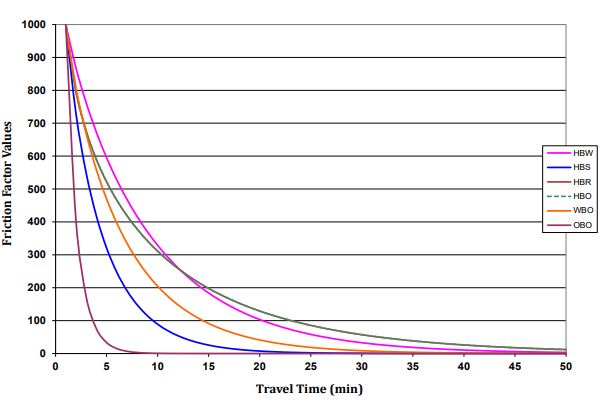
This figure shows the curve of impedance function calibrated for each trip purpose. — **Figure 11.2** Friction factor distribution by trip purpose. From Lincoln travel demand model, by Lima & Associates, p.89, 2011, In the Public domain.

In very general terms, a friction factor F_ij that is an inverse function of travel impedance W_ij is used in trip distribution to plug in the travelers’ willingness to travel between zone i and zone j.

$F_{ij} = \frac{1}{W_{ij}}$

K-Factor

Travel demand modeling is influenced by various socio-economic factors that affect travel behavior and demand for different purposes. Chapter 10 highlights the most significant factors in travel demand modeling: income, auto ownership, availability of multimodal transportation systems, age, and job type (Pan et al., 2020). Therefore, the K-Factor method was developed and plugged into the gravity model to represent variation in socio-economic factors and adjust interzonal trips accordingly. For example, a blue-collar employee working in a low-income suburb may exhibit different travel behaviors (in terms of mode choice and frequency of travel) compared to a white-collar employee working in the central city with a higher income. The K-factor is determined and plugged into the gravity formula to accommodate such differences.

Recall the classic land use models presented in Chapter 4. Based on the proximity to employment centers or the central business districts, different neighborhoods offer housing and job options tailored to individuals in different income brackets. For example, the earnings of employees in chain restaurants significantly contrast with those working in Central Business District (CBD) headquarters. Prevailing land use policies and the typical American development pattern heighten this disparity. Consequently, these groups are likely to inhabit geographically distant areas in a country like the United States. Furthermore, people of varying income levels or social statuses may respond differently to travel impediments, such as travel time or cost.

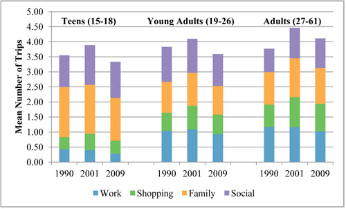
Calibration of K values is determined by comparing the estimated results and observed data for the base year (Tawfik & Rakha, 2012). The K numeric value will be above one (>1) if the socio-economic factors contribute to more travel and less than one (< 1) if otherwise (Meyer, 2016). Figure 11.3 shows the mean number of trips for different age groups (K-factor) and various trip purposes. Accordingly, calculating friction factors and K-factors for different purposes and socio-economic groups yields a better fit to the data.

number of trips by age for work, shopping, family and social for three years. — **Figure 11.3** Mean number of trips by purpose and age group From Trip Purpose by FHWA, 2023, https://www.fhwa.dot.gov/policy/otps/nextgen_stats/chap7.cfm. In the Public Domain.

11.2.3 Example 1

Consider a small area with three zones (TAZs). Table 11.1 shows the trip generation results for each zone, and Table 11.2 shows the travel time for each pair of zones. The friction factor is also given in this example as a function of travel time in Table 11.3. The intrazonal travel time for zone 1 is larger than that of most other inter-zone times because of the geographical characteristics of the zone and lack of access within the area. Using this information, please calculate the number of trips for each pair of zones.

Solution:

For the calculation of trip distribution between the three zones, the trip generation and attraction table from step one of the FSM model is the input data, and then the gravity model is used for calculation. Tables 11.1, 11.2, and 11.3 represent the trip generated and attracted for each zone, travel time between each pair of zones, and friction factor derived from the travel time.

**Table 11.1** Trip Generation Results.
TAZ	1	2	3	total
Trips Productions	220	245	305	770
Trip Attractions	210	270	350	770

**Table 11.2** Travel Time Matrix.
TAZ	1	2	3
1	6	4	2
2	4	5	4
3	2	4	5

**Table 11.3** Travel time and Friction Factor.
Travel Time	FF
1	82
2	52
3	50
4	41
5	35
6	26
7	20
8	13
9	9
10	5

Now with this information, we can start the calculation process. First, we have to estimate the attractiveness of each zone using the equation (1)

For example, for zone 1 we have:

Attractiveness1= 210*26=5460

Attractiveness2= 210*35=7350

Attractiveness3= 350*35=12250

Now, we use the pivotal formula of the gravity model (equation 2). Accordingly, we have (K-factor set to 1):

$T_{1-1}=220\times\frac{210\times26}{(210\times26) (270\times41) (350\times52)}$ =35

$T_{1-2}=220\times\frac{270\times41}{(210\times26) (270\times41) (350\times52)}$ =70

$T_{1-3}=220\times\frac{350\ast52}{(210\times26) (270\times41) (350\times52)}$ =115

$T_{2-1}=245\times\frac{210\ast41}{(210\times41) (270\times35) (350\times41)}$ =65

$T_{2-2}=245\times\frac{270\times35}{(210\times41) (270\times35) (350\times41)}$ =71

$T_{2-3}=245\times\frac{350\times41}{(210\times41) (270\times35) (350\times41)}$ =108

$T_{3-1}=305\times\frac{210\ast52}{(210\times52) (270\times41) (350\times35)}$ =97

$T_{3-2}=305\times\frac{270\times41}{(210\times52) (270\times41) (350\times35)}$ =98

$T_{3-3}=305\times\frac{350\times35}{(210\times52) (270\times41) (350\times35)}$ =109

The result of the calculation is summarized in Table 11.4:

**Table 11.4** Trip distribution results.
TAZ	1	2	3	Calculated	Observed
1	35	70	115	220	200
2	65	71	108	244	248
3	97	98	109	304	320
Calculated	197	239	332	768	768
Observed	210	288	270	768

However, our calculations’ results do not match the already existing and observed data. The mentioned mismatch is why calibration and balancing of the matrix are needed. In other words, we must perform more than one iteration of the model to generate more accurate results. For performing a double or triple iteration, we use a formula discussed at the end of this chapter (example adapted from: Garber & Hoel, 2018).

Growth Factor Model

After successfully calibrating and validating the data we have estimated, we can also apply the gravity model to forecast future travel behavior or travel patterns in our study area. Future trip distributions can be predicted by using the change in land-use data, socioeconomic data, or any other changes in the whole system. We can calculate trip distribution from the O-D table for either base or forecasting year when the friction factor and K-factor data are unavailable or unsatisfactorily calibrated. Depending on historical trends and data, growth factor models are limited if an observed O-D table is unavailable. Similar to the trip generation step, growth factor models cannot incorporate updated travel time as the change in travel time between zones can highly affect travel patterns (Qsim, 2016).

Fratar method

One of the most common mathematical formulas of the growth factor model is the Fratar method, shown in the following equation. Through his method, the future distribution of trips from one zone is equal to the present distribution multiplied by the growth factor of the destination zone between now and the forecasting year (Heanue & Pyers, 1966). The formula to calculate future trip values is shown in equation below:

$T_{ij}=\left(t_iG_i\right)\frac{t_{ij}G_j}{\sum_{x}\hairsp\hairsp t_{ix}G_x}$

where:

T_ij =number of trips estimated from zone to zone
t_i =present trip generation in zone
G_x =growth factor of zone
T_i =future trip generation in zone
t_ix =number of trips between zone and other zones
t_ij =present trips between zone and zone
G_j =growth factor of zone

The following section will discuss an example illustrating the application of the Fratar method.

Example 2

The case study area of this example consists of four TAZs. Table 11.5 shows the current trip distributions. Assuming the growth rate for each TAZ is shown in Table 11.6, the next step is to calculate the number of trips between each two TAZs in the future year.

**Table 11.5** Current trip distribution.
TAZ	A	B	C
A	n/a	300	200
B	150	n/a	100
C	100	200	n/a
Total	250	500	300

**Table 11.6** Current trip distribution.
TAZ	Total Generation	Growth Factor	Total Generation for Forecasting Year
A	250	1.3	325
B	500	1.5	750
C	300	1.1	330

To solve this problem, apply the Fratar Method using the required two estimates for each pair. These estimates should be averaged; the resulting value will be the final T_ij. Based on the formula, calculations are as follows:

$T_ij =(t_i G_i ) (t_ij G_j)/(∑_x t_ix G_x )$

$T_A_B =(250*1.3 ) (300*1.3)/((300*1.5) (200*1.1))=218$

$T_B_A =(500*1.5)(150*1.3)/(150*1.3) (100*1.1))=480$

$T_(mean)_A_B =(T_A_B T_B_A)/2=(261 960)/2=349$

$T_A_C =(250*1.3 ) (200*1.1)/((300*1.5) (200*1.1))=107$

$T_C_A =(300*1.1)(100*1.3)/(100*1.3) (200*1.5))=99$

$T_(mean)_A_C =(T_A_C T_C_A)/2=(107 99)/2=103$

$T_B_C =(500*1.5 ) (100*1.1)/((100*1.1) (150*1.3))=270$

$T_C_B =(300*1.1)(300*1.3)/(200*1.5) (100*1.3))=300$

$T_(mean)_B_C =(T_B_C T_C_B)/2=(270 300)/2=349$

Based on the calculations, the first iteration of the method will yield the following table:

**Table 11.7** Estimated trip distribution using Fratar formula.
TAZ	A	B	C	Estimated Total Generation	Actual Total Generations
A	n/a	349	103	452	490
B	349	n/a	285	634	600
C	103	285	n/a	388	420
Total	452	500	300

To estimate future trip rates between zones, use the Fratar formula, as shown in Table 11.7. However, there is a problem with the estimated total number of trips generated in each zone not being equal to the actual trip generation. Therefore, a second iteration is necessary. In this second iteration, we use the new O-D matrix as the input to calculate new growth ratios. The trip generation is estimated to occur in the next five years based on the preceding calculation. As an exercise, you can conduct as many iterations as needed to bring the estimated and actual trip generations into alignment.

Example 3

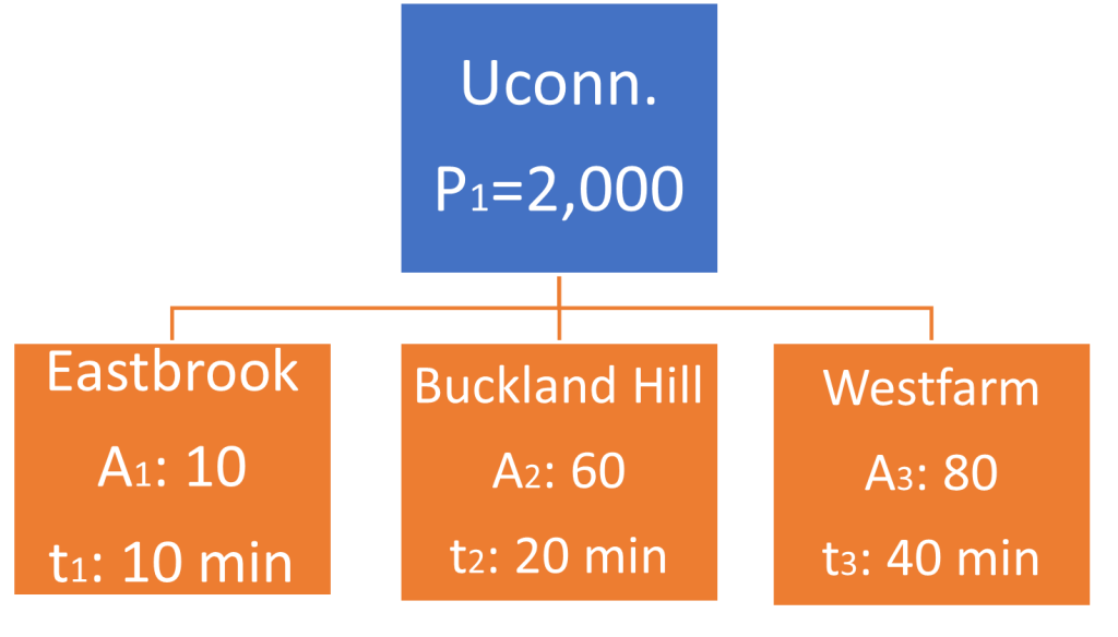
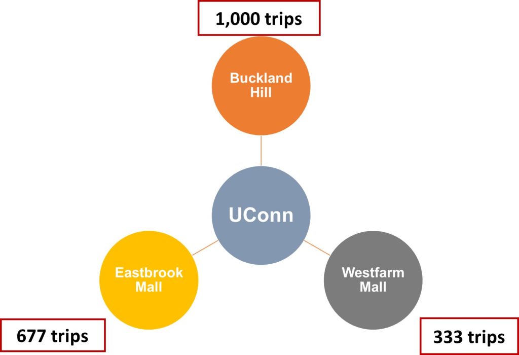
In a hypothetical area, we are interested in determining the number of trips attracted by three different shopping malls at various distances from a university campus that generates about 2,000 trips per day. In Figure 11.4, the hypothetical area, the number of trips generated by the campus, and the total number of trips attracted for each zone are presented:

This figure shows the trip generator and the three possible destination with their travel time. — **Figure 11.4** Schematic Orientation of Trip Generation zone and Trip Attracting Zones.

socioeconomic adj. Factor K=1.0
Calibration factor C=2.0

Solution

As the first step, we need to calculate the friction factor for each pair of zones based on travel time (t). Given is the following formula with which we calculate friction factor:

$F_{1j} = t_{ij}^{-2}$

Next, using the friction factor, we use the gravity model to calculate the relative attractiveness of each zone. In Table 11.8 , you can see how calculations are being carried out for each zone.

**Table 11.8** Calculation of trip distribution (Friction Factor and Relative Attractiveness).
J	Aj	t1j	F1j=tij^(-2)	Aj*F1j
1	10	10	1/100=0.01	0.1
2	60	20	1/400=0.0025	0.15
3	80	40	1/1600=0.000625	0.05
Total				0.3

**Table 11.9** Calculation of Final trip distribution.
J	Aj*F1j	P1j=	T1j= P1*p1j
1 (Eastbrook Mall)	0.1	0.1/0.30=0.333	2,000*0.33=667
2 (Buckland Hill)	0.15	0.15/0.3=0.5	2,000*0.5=1,000
3 (Westfarm Mall)	0.05	0.05/0.3=0.167	2,000*0.167=333
Total	0.3	1	2000

Next, with having relative attractiveness of each zone (or probability of attracting trips), we plug in the trip generation rate for the campus (6,000) to finally estimate the number of trips attracted from the campus to each zone. Figure 11.5 shows the final results.

This figure shows the results of example 3 graphically. — **Figure 11.5** Final Results.

Model Calibration and Validation

Model validation is an integral part of all simulation and modeling procedures. One of the most essential steps in FSM modeling is developing a procedure to calibrate its final outputs (predictions) with actual and observed data. To do this, model parameters are adjusted so that the observed data and estimations have fewer mismatches (Meyer, 2016). After such adjustments, the model with calibrated parameters can help in simulation and future scenario analyses.

After completing the trip distribution step, it is important to compare model calibration and adjustment results in each category (i.e., by trip purpose) with recorded real-world trips from the O-D survey.

If the two values are not identical, model parameters, like FF or K-factors, are reassigned and re-run the gravity model. The process continues until the observed data and estimations are very close (ratio between 0.9 and 1.1).

The following example shows the process of trip distribution step with calibration.

11.4.1 Example 4

This example demonstrates the calibration process. The first step is to identify the model’s inputs, which are the outcomes of the trip generation process. The following tables show the results obtained from surveys and actual trip data, as well as the travel time between each pair of zones (represented by the friction factor (FF)) and the socioeconomic conditions (Tables 11.10, 11.11, and 11.12 ). The column with the heading “A’ “in Table 11.11 represents observed generated trips.

**Table 11.10** Travel Time Matrix.
Travel Time Matrix	blank cell
Zone	1	2	3
1	1	6	11
2	7	3	12
3	15	13	4

**Table 11.11** Trip Generation Results.
Outcomes of trip generation	blank cell	blank cell	blank cell
Zone	P	A	A’
1	550	440	400
2	600	682	620
3	380	561	510
	1530	1683	1530

**Table 11.12** FF Matrix.
Friction Factors	blank cell
Zone	1	2	3
1	0.876	1.554	0.77
2	1.554	0.876	0.77
3	0.77	0.77	0.876

**Table 11.13** K-factor Matrix.
K Factors	blank cell	blank cell	blank cell
Zone	1	2	3
1	1.04	1.15	0.66
2	1.06	0.79	1.14
3	0.76	0.94	1.16

here are several formulas, such as negative exponential or inverse power function, that can be used to calculate friction factors from impeding factors like travel cost or time, as discussed in previous sections. To estimate the number of trips between each pair of zones, we use the gravity formula and input the necessary data. Table 11.14 shows the results of trip distribution for each pair of zones. However, the total number of trips attracted from our calculations is different from observed data.

**Table 11.14** Trip Distribution Results.
Zone	1	2	3	produced
1	116	352	82	550
2	257	168	175	600
3	74	142	164	380
attracted	447	662	421
	400	620	510

Now, by looking to the last table we can see that the total number of trips produced is exactly matching to the results of the trip generation table. But the total attractions and actual data have a mismatch. In the next step, we apply the calibration methods in order to make our final results more accurate.

Row F.

**Table 11.15** First iteration by row (correct for generation).
Zone	1	2	3	blank cell
1	104	330	100	533	1.031849
2	230	157	212	599	1.001418
3	66	133	199	398	0.955191
	400	620	510

In the first iteration of calibration, we have to generate a value called column factor, which is the result of dividing actual data attraction by estimated attractions. Then we apply this number for each pair in the same column. In Table 11.15, we can observe that the sum of attractions is now the same as the actual data, but the sum of generation amounts is now different from actual data generation. In this step, we perform another iteration, the same as the first iteration but instead of column factor, we plug in row factor value, which is the result of dividing actual data trip generation by estimated generation.

**Table 11.16** Second Iteration by Column (Correct for attraction).
Zone	1	2	3	blank cell
1	107	340	103	550
2	231	157	212	600
3	63	127	190	380
	401	625	505
Col. F	0.998364	0.992373	1.010743

A third iteration is needed because the sum of attraction is still different from the actual data, and we must generate another column factor. The results are shown in Table 11.17.

**Table 11.17** Third iteration by column (correct for attraction).
Zone	1	2	3	blank cell
1	107	338	104	548
2	230	156	214	601
3	63	126	192	381
	400	620	510

Based on the results of the third iteration results, we see the attractions are now accurate, and trip generations have very insignificant differences with actual data. At this point, we can stop the calibration. However, the procedure can continue to calibrate results to decrease the difference as much as possible. In other words, the sensitivity of the calibration, the threshold for the row and column factors, can be adjusted by the modeler.

Conclusion

In this chapter, we demonstrated the procedure, application and other details of the second step of FSM modeling framework. Using the concept of gravity-based accessibility, we saw how the production and attraction table can be transformed into a trip distribution matrix. By using simple numerical examples, we showed how different methods can be applied to calculate trips between pair of zones. Assumption of homogenous behavior, assumption of static and sequential behavior, aggregation biases, and less emphasis on lots of social and physical barriers. Dynamic modeling (concurrent mode and destination choice), micro-simulation, agent-based models or newer methods such machine learning have made several enhancement to the traditional model. Collection of real-time data as well as increase in computational capacity has opened such prospects in travel demand modeling and trip distribution studies.

Glossary

Emissivity is a quantity that represents the trip production rate of a neighborhood, similar to attractiveness for trip attraction.
Intra zonal trips are those trips that both ends of the trip is in the same zone.
Interzonal Trips are those trips where one end of the trip is in a different zone.
Uniqueness is a quantity defined for a TAZ that indicates how unique that zone or trip attraction center is.
Gamma distribution is a probability distribution that is used for converting travel times into impedance functions
Blue-collar employee is a worker who usually performs manual and low-skill duties for their work.
White-collar employee is a worker who is high-skill and performs professional, or administrative work.
Zonal Emissivity refers to a quantity that represents the trip making rates for that zone. Factors affecting this feature can be population, employment, income level, vehicle ownership, etc.

Key Takeaways

In this chapter, we covered:

What trip distribution is and the factors that determine attractiveness of zones for travel demand.
Different modeling frameworks appropriate for trip distribution and their mathematical formulation.
What advantages and disadvantages of different methods and assumptions in trip distribution are.
How to perform a trip distribution manually using simplified transportation networks.

Prep/quiz/assessments

What factors affect the attractiveness of the zones in trip distribution, and what input data is needed to measure such attractiveness?
What are the advantages and disadvantages of the three trip distribution methods (gravity model, intervening opportunities, and Fratar model)?
What are the friction factor and K-factor in trip distribution, and how do they help to calibrate model results?
How should we balance trip attraction and production after performing trip distribution? Explain.

References

Allen, B. (1984). Trip distribution using composite impedance. Transportation Research Record, 944, 118–127.

Seggerman, KE. (2010). Increasing the integration of TDM into the land use and development process. Fairfax County (Virginia) Department of Transportation, May. Department of Transportation.

Cesario, F. J. (1973). A generalized trip distribution model. Regional Science Journal, 13(2), 1973-08

Council, A. T. (2006). National guidelines for transport system management in Australia 2006. Australia Transportation Council. https://www.atap.gov.au/sites/default/files/National_Guidelines_Volume_1.pdf

Garber, N. J., & Hoel, L. A. (2018). Traffic and highway engineering. Cengage Learning.

Hansen, W. G. (1962). Evaluation of gravity model trip distribution procedures. Highway Research Board Bulletin, 347. https://onlinepubs.trb.org/Onlinepubs/hrbbulletin/347/347-007.pdf

Ned Levine (2015). CrimeStat: A spatial statistics program for the analysis of crime incident locations (v 4.02). Ned Levine & Associates, Houston, Texas, and the National Institute of Justice, Washington, D.C. August.

Lima & Associates. (2011). Lincoln travel demand model. Lincoln Metropolitan Planning Organization. (2011). https://www.lincoln.ne.gov/files/sharedassets/public/planning/mpo/projects-amp-reports/tdm11.pdf

Meyer, M. D. (2016). Transportation planning handbook. John Wiley & Sons.

NHI. (2005). Introduction to Urban Travel Demand Forecasting. In National Highway Administration (Ed.), Introduction to Urban Travel Demand Forecasting. American University.. National Highway Institute : Search for Courses (dot.gov)

Pan, Q., Jin, Z., & Liu, X. (2020). Measuring the effects of job competition and matching on employment accessibility. Transportation Research Part D: Transport and Environment, 87, 102535. https://doi.org/10.1016/j.trd.2020.102535

PE Lindeburg, M. R. (2017). PPI FE civil review – A comprehensive FE civil review manual (First edition). PPI, a Kaplan Company.

Qasim, G. (2015). Travel demand modeling: AL-Amarah city as a case study. [Unpublished Doctoral dissertation , the Engineering College University of Baghdad]

Tawfik, A. M., & Rakha, H. A. (2012). Human aspects of route choice behavior: Incorporating perceptions, learning trends, latent classes, and personality traits in the modeling of driver heterogeneity in route choice behavior. Virginia Tech Transportation Institute. Blacksburg, Virginia https://vtechworks.lib.vt.edu/handle/10919/55070

Thill, J.-C., & Kim, M. (2005). Trip making, induced travel demand, and accessibility. Journal of Geographical Systems, 7(2), 229–248. https://doi.org/10.1007/s10109-005-0158-3

Verlinde, E. (2011). On the origin of gravity and the laws of Newton. Journal of High Energy Physics, 2011(4), 1–27. https://link.springer.com/content/pdf/10.1007/JHEP04(2011)029.pdf

License

Icon for the Creative Commons Attribution-NonCommercial-ShareAlike 4.0 International License

Transportation Land Use Modeling and Policy (TLUMP) Copyright © 2024 by Qisheng Pan and Soheil Sharifi is licensed under a Creative Commons Attribution-NonCommercial-ShareAlike 4.0 International License, except where otherwise noted.