12 Third Step of Four Step Modeling (Mode Choice Models)
Chapter Overview
Mode choice is the third step of traditional Four-Step Modeling (FSM). Mode choice models are used to analyze and predict the choices of individuals or groups in selecting transportation modes for types of trips. The goal of the model is to predict the shares, or the absolute number of trips, made by each mode. An important objective in mode choice modeling is to predict the share of trips in public transportation. Chapter 12 first introduces the factors affecting individuals’ mode choice. It then elucidates different types of mode choice or modal split analysis. This chapter explains the properties, the required steps, and the mathematical formulas of mode choice models. The calculations of mode choice are demonstrated with examples at the end of the chapter.
Learning Objectives
- Define the mode choice model’s role in FSM and its importance for a complete travel demand model.
- Summarize the factors that influence the mode choice of travelers and explain how to incorporate them into the model.
- Compare different modeling frameworks for modal split analysis and summarize their strengths and weaknesses.
- Solve modal split analyses manually for small samples using the discrete choice modeling framework and multinominal logit models.
Introduction
We delved into the first two steps of FSM (Four-Step Model) in earlier chapters, exploring trip generation, attractions, and distribution modeling through relevant models and frameworks. This chapter focuses on the third phase of FSM, specifically, mode choice modeling and provides a general definition of this step, outlines its key objectives, and offers a brief historical overview of the model.
While trip distribution yields a matrix of origin-destination (O-D), this step disaggregates the total number of O-D trips by mode, also known as modal share. The Chicago Area Transportation Study (CATS) developed one of the earliest versions of choice modeling (CATS, 1959). The primary purpose is to know how many travelers used public transit to travel into the CBD (Central Business District) and how many used it for local trips. After CATS, London adopted the same methodology and divided the trips into two types – trips in the inner city and trips in the outer parts. The London version also assumed an income implication for mode choice as certain income levels could purchase private cars (Levinson et al., 2014).
Mode selection is a complex process done by the traveler based on individual logical decisions. The potential factors that affect travelers’ decisions are their income level, availability of public transit, auto ownership rate, and the relative utility of each mode in terms of costs, time, safety, and convenience. As a result, the mode choice model attempts to replicate individual travel behavior based on individual factors, the transportation system, and the type of trip (Barff et al., 1982; Ben-Akiva & Lerman, 1974; Swait & Ben-Akiva, 1987).
Modal split is a crucial component of the FSM model as it determines the number of private car trips taken on weekdays. Accurately determining transportation trends is essential for planners to predict congestion, forecast future trends, and efficiently allocate traffic to the network. Many transportation policies and programs aim to encourage a shift from cars to more sustainable modes, such as biking or riding transit. Mode choice models can generate results that evaluate the effects of policies on such modal shifts. For instance, in a case where private car usage turns out to be significant in a city based on the results from the mode choice modeling, planners may suggest implementation of use tolls on a specific part of the network to persuade drivers to use other more sustainable transportation modes.
There are multiple methods for formulating mode choices in transportation. Discrete choice models (Ben-Akiva & Bierlaire, 1999) are currently the most dominant and frequently used models in transportation mode choice. Commonly used in practice, multinomial and nested logit models are the predominant modeling approach. Of the multinomial logit models, discrete-outcome modeling approach is the most widely used (Bhat, 1995; McFadden et al., 1977), and is based on the concept of utility. Before elaborating on discrete choice models and their application in transportation mode choice, we introduce some earlier models of mode choice in transportation in the following section.
Diversion Curve Techniques
In transportation, CATS first used diversion curve techniques for some tasks. In the beginning, CATS was interested in estimating how much diversion would occur from local roads to newly built expressways and bypasses built around the city. This method’s formula for mode choice is presented in equation (1):
 (1)
(1)
where,
cm is travel time by mode m and,
R is empirical data in the curve
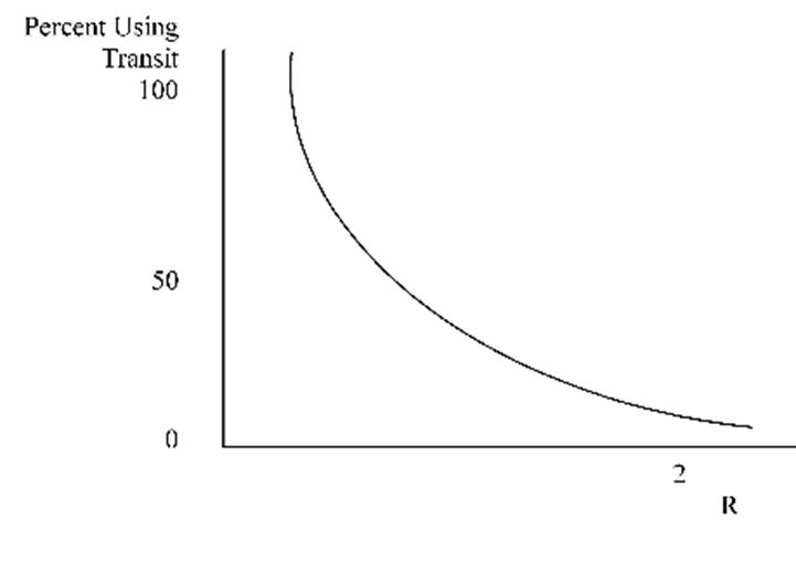
Figure 12.1 depicts the percentage of users in the market that choose transit based on “R”. For building this curve, travel cost can also be used as a representation of travel impedances. Therefore, the less the degree of impedance, the greater the percentage of transit use. The diversion curve has been used to explain different conditions, and supplementary variables, like income or density, are implicit in the model. This method can also be used to estimate diversion to other routes or departure times (Levinson et al., 2014).
Discrete Choice Modeling
Transportation modes are the alternative means that travelers choose based on the maximization of their utility. These options (modes) are separate (discrete) from each other. Economics was the first field to apply this model. Using discrete choice models helps the modeler to predict the choice between several options, such as working for a firm or not or choosing between different transportation modes. In contrast with standard consumption models, where the variables are continuous, regression analysis can help forecast continuous value, discrete choice models. The results are the probability of choosing each discrete choice.
The model’s development can be traced back to McFadden’s (1973) research and other researchers, who formulated the problems of travel mode and location decisions as microeconomic consumer choice problems among distinct alternatives. Before McFadden’s work, there was a decade of empirical research based on binary choice analysis (Warner, 1962). Much like the empirical research on gravity models, the work on choice modeling preceding McFadden’s contributions failed to provide theoretical grounding of empirically established concepts. McFadden’s derivation of the logit model from utility maximization closed this gap, and a new area of research, labeled “behavioral demand modeling,” emerged. It stresses using stochastic utility maximization and disaggregated small-sample data in estimating choice models via maximum likelihood. Later in this chapter, a more detailed exploration of discrete choice modeling will be presented (Koppelman, 2007).
As we discussed earlier, transportation modes are the alternatives that travelers choose based on the maximization of their utility, and these options (modes) are separate (discrete) from each other. In economics (the first field that applied this model), discrete choice models help the modeler to predict the choice between several options, such as working for a firm or not or choosing between different transportation modes. In contrast with standard consumption models, where the variables are continuous, and regression analysis can help us forecast continuous value, discrete choice models result in the probability of choosing each discrete choice.
The development of this model originated in the work of McFadden (1973) and others. They began with formulating the problems of travel mode and location decisions as problems in microeconomic consumer choice among discrete alternatives. A decade of empirical research stemming from binary choice analysis preceded McFadden’s work (Warner, 1962). “Much like the empirical research on gravity models, the work on choice modeling preceding McFadden’s contributions had failed to provide a theoretical grounding of empirically established concepts. McFadden’s derivation of the logit model from utility maximization closed this gap, and a new area of research, labeled “behavioral demand modeling,” emerged” (Anas, 1983). It stresses using stochastic utility maximization and disaggregated small-sample data in estimating choice models via maximum likelihood. Later in this chapter, a more detailed exploration of discrete choice modeling will be presented (Koppelman, 2007).
Factors Affecting Transportation Alternative Choices
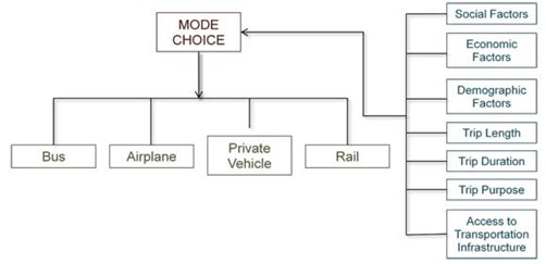
As we all have experienced choosing between different transportation modes for our destinations, discrete choice models also encompass all such choices in the models. In a multimodal transportation system, various modes (such as biking, walking, transit, private car, shared cars, etc.) are available. The hierarchy of such choices are shown in Figure 12.2:
Many alternative modes are available for an individual to travel from one place to another, such as driving alone or with someone else, walking, taking the train, bus, taxi, riding a bicycle, etc. Many factors affect individual mode choice.
When choosing a mode of transportation from one location to another, travel behavior is influenced by factors such as the characteristics of the traveler, trip features, and transportation system features (Meyer, 2016). The model incorporates variables such as automobile ownership, income, number of workers per household, and the distance between the origin and destination to characterize travelers. For instance, students living close to campus at a university may choose to walk or bike to the university daily. In contrast, commuter students from further areas may opt for private cars or take the bus or train.
A second set of factors to consider when planning a trip are the trip features. These include the trip’s purpose, length of journey, starting and ending locations, and time of day. For instance, an individual may choose to take public transportation to get to work but opt for a different mode of transportation when running errands. The third category of variables is related to the attributes of the transportation system. These variables include travel costs, travel time, comfort level, convenience, reliability, and security of different modes. For instance, an increase in bus fares may cause people who ride buses to switch to private vehicles. Similarly, a rise in parking fees may lead some people who currently drive to work to switch to other modes of transportation.
The fourth category that determines mode choice for travelers includes zonal characteristics. The variables in this category can be residential density and workforce density. For instance, public transit ridership increases as road congestion increases.
The final set of factors that influence mode selection relates to network features. The group ratio is determined by comparing the value of the variable for public transit to that of the same variable for a private car. Among these variables, the access ratio, travel time ratio, and travel cost ratio are the most significant and decisive determinants of the mode of transportation people choose.
Types of Mode Choice Models
In the context of U.S. cities, most trips are made by private car, despite an understanding about the importance of multimodal systems and transit ridership for daily trips. Accordingly, several mode choice models are solely interested in calculating the share of trips between auto and transit. Three models for doing so are (1) direct generation of transit trips, (2) use of trip end models, and (3) trip interchange modal split models.
12.4.1 Direct Generation Models
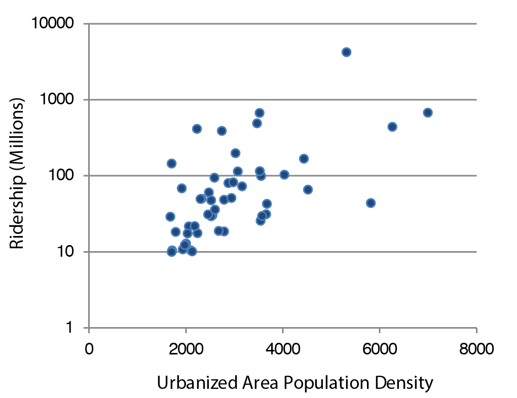
As mentioned, transit trips are under the influence of auto availability and population density (which determines the feasibility of riding transit). Figure 12.3 illustrates the relationship between population density, and transit ridership. According to the figure, as density grows, transit ridership increases.
The following example shows how to use direct generation models for estimating transit trips.
Example 1
A zone with an area of 20 acres accommodates 4,000 people. Fifty percent of households have no access to a car, and the other half have one auto per household. With this information, determine the number of transit trips per day in this zone.
Solution: First, we need to calculate population density:
Population density = 4000/20 = 200
Calculate the number of persons per acre: 5000/50 = 100. Then determine the number of transit trips per day per 1,000 persons (from Figure 12.3) to calculate the total of all transit trips per day for the zone.
Zero autos/HH: 320 trips/day/1000 population
One auto/HH: 250 trips/day/1000 population
Total Transit Trips: (0.50)(510)(4) + (0.50)(630)(4) = 1020 + 1260 = 2280 transit trips per day (example adapted from Qasim, 2012)
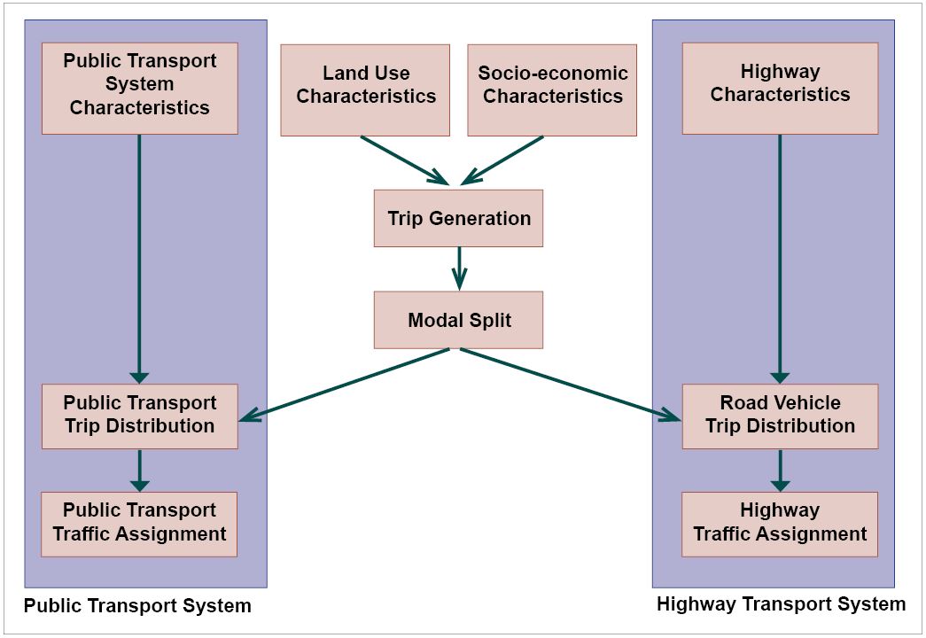
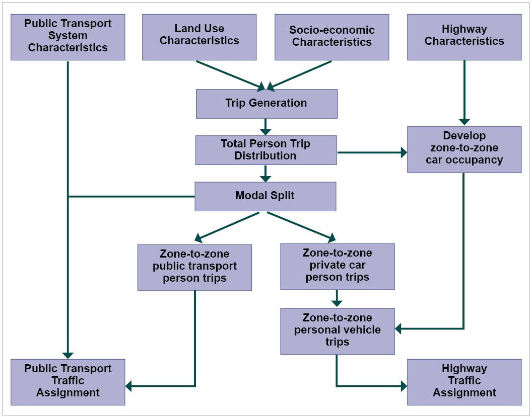
Trip End Models
Like the direct generation model, the trip end model is also indifferent to transportation network variables such as network quality. To calculate person trips, this model performs immediately after trip generation (first step). This model considers personal characteristics as the most important determinant of mode choice. Although this mode is effective for short trips, it fails to account for changes in the transportation system, such as new charging schemes and roadway extensions (Mathew & Rao, 2006).
Figure 12.4 shows this model’s relative location in the FSM model’s structure.
The general procedure for this model is as follows:
- Calculate the total trip production and attractions.
- Calculate the urban travel factor.
- Estimate the total number of transit trips using mode choice curve.
- Determine the vehicle occupancy rate.
- Distribute the travel demand for auto and transit separately.
The following example is an estimation of modal split using the trip end model:
Example
In a hypothetical zone, the total trips generated are 8,000 trips per day. The average number of automobiles per household is 2.2, and the population density is equal to 12,000 persons per square mile. What is the share of travelers who are expected to ride transit?
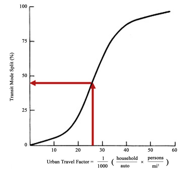
Solution: Compute the urban travel factor.
UTF= 26.4
26.4
From the figure (12.5), we can state that it is expected that transit trips comprise around 47% of total trips (example adapted from Garber & Hoel, 2018).
12.4.5 Trip Interchange Models
Unlike the trip-end model, this method estimates a modal split after trip distribution. Also, another important difference of this method compared to the previously mentioned models is that it considers system level-of-service variables, including travel time or travel cost.
The mathematical formula for this model is shown in equations (2):
The mathematical formula for this model is shown in equations (2):
 or,
or,

 (2)
(2)
where:
MSt= the share of trips between the two zones
MSa = the share of trips between the two zones made via auto
Iijm = a measure of travel impedance between the two zones, which is a representation of the total cost associated with this trip. [Impedance = (in vehicle time min) + (2.5 * excess time min) + (3 * trip cost, $ / income earned/min).] (In this model, in-vehicle time refers to the amount of time spent in the car while traveling, and excess time is the time out of the vehicle, such as waiting in the stations or switching lines.)
b = an exponent, which depends on trip purpose
m = t for transit mode; a for auto mode
Figure 12.6 shows the relative location of this model in the structure of FSM model.
The input data needed for this model is:
- Distance between zones
- Transit fare,
- Private Auto out-of-pocket costs,
- Parking costs,
- Highway and transit speed limit
- Model parameters (b)
- Income,
- Excess time
Example 3 illustrates how the trip interchange model can be used for mode choice estimation.
Example 3
Zone S is designated as a suburban zone and Zone D is the CBD zone. Table 12.1 shows the distance and travel costs between the two zones. Using this information, determine the share of each mode. B is equal to 2, and the median income is $30,000 per year.
Assume that the data shown in Table 12.1 has been developed for travel between a suburban zone S and a downtown zone D. Determine the percentage of work trips by auto and transit. An exponent value of 2.0 is used for work travel. Median income is $24,000 per year.
| blank cell | Auto | Transit |
|---|---|---|
| Distance | 12 mi | 7 mi |
| Cost per mile | $0.20 | $0.16 |
| Excess time | 4 min | 9 min |
| Parking cost | $1.50 (or 0.75/trip) | – |
| Speed | 30 mi/h | 20 mi/h |
Solution
Using equation (2), we have:
![I_S_D_a=\left(\frac{12}{30}\times60\right)+\left(2.5\times12\right)+\left\{\frac{3\times\left[\left(\frac{1.50}{2}\right)+0.15\times12\right]}{\frac{30,000}{120,000}}\right\}=84.6](https://uta.pressbooks.pub/app/uploads/quicklatex/quicklatex.com-c1a2530774a678a42b002c040b7d703a_l3.png "Rendered by QuickLaTeX.com")
![I_S_D_t=\left(\frac{7}{20}\times60\right)+\left(2.5\times7\right)+\left[\frac{3\times\left(7\times0.16\right)}{\frac{30,000}{120,000}}\right]=51.94](https://uta.pressbooks.pub/app/uploads/quicklatex/quicklatex.com-5a100f29669c0beca9fd86476b150a43_l3.png "Rendered by QuickLaTeX.com")


Thus, the mode choice of travel by transit between Zones S and D is 27.3%, and by highway the value is 72.6%. These shares can be multiplied by the total number of trips between the two zones to calculate the number of trips by auto and transit (example adapted from Garber & Hoel, 2018).
12.5 Logit Models
Among all models developed for mode choice estimation for urban trips, the logit model and application of the utility function are the most popular and dominant methods of forecasting modal share. The remainder of the chapter will explain this concept, formula, and related examples.
Logit models can be considered as both aggregate and disaggregate models. They are aggregate models because they provide a single value that describes the traveler’s choice in the region. However, the model also uses the concepts of discrete choices and utility maximization from both psychology and economics and thus can also be considered disaggregate models because they analyze individuals as the unit of analysis (Levinson et al., 2014).
12.5.1 Psychological and Economic Roots of Discrete Choice Model
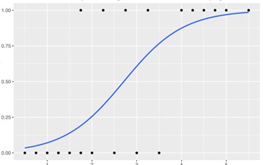
A simple psychological experiment can explain discrete choice models. Suppose we compare two objects with weights, w1 and w2. What is the probability of choosing the heavier one correctly? It is very rational to think that the more different the weights are, the higher the chance of choosing the correct one. Figure 12.7 shows the relationship between the difference in weights (horizontal axis) and correct choice probability (vertical axis).
In econometrics, however, the issue is about utility rather than the perceived weights of objects or similar things. In econometrics, the utility function can be written as equation (3):
observed utility = mean utility + random term (3)
Taking into account the features of object x (the ones that affect its utility such as a housing unit area when choosing between housing options), we have in equation (4):

Here, we assume that the error term (uncertainties) is distributed independently and identically with a Weibull, Gumbel type I, or double exponential distribution. This assumption yields us a model of multinomial logit model (MNL). The logit model is determines the log ratio of the probability of choosing a mode vs the probability of not choosing that particular mode, as shown in the equation (5):


 (5)
(5)
Before we continue to describe the model and its formulas, it would be beneficial to look at how this concept can help transportation planners determine the modal split. To that end, Figure 12.8 is designed to show how the model is structured for the transportation modal split.
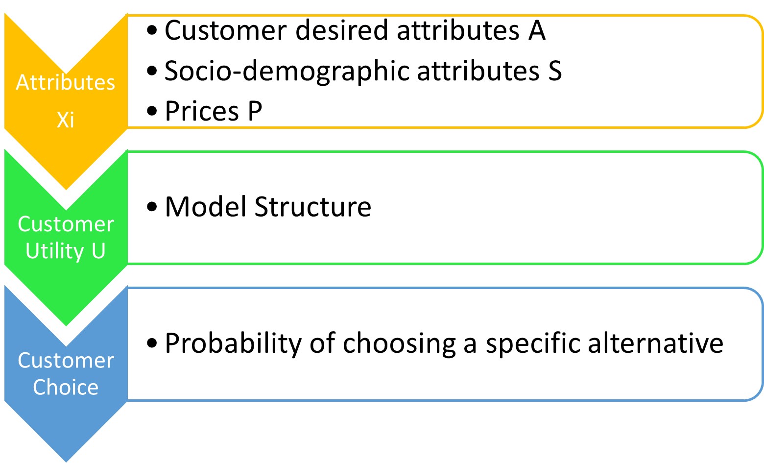
Note. Figure created by Authors.
In this figure, as you can see, the input for the model comes from the attributes that we discussed earlier in this chapter. Travelers’ behaviors, socio-demographic characteristics and costs are attributes that yield us with a utility function. Next, using this function we can estimate the portion of each transportation mode usage from the probability distribution of logit models.
Utility Function
Discrete choice models assume travelers make rational decisions. This assumption suggests that people make decisions that maximize their utility based on the information available to them at the time of decision, according to the rational choice theory (Hechter & Kanazawa, 1997). The variables defining the utility function are considered random due to heterogeneity in preferences, calculation errors, unobserved attributes, and insensitivity to small changes in attributes. The utility function indicates the value of each choice for the traveler in terms of utility (McFadden, 1980). For instance, mode M will be chosen by the traveler if the utility of M is greater than the utility of all other modes. However, utility functions can be subject to uncertainties due to the availability of data and the lack of knowledge about the traveler’s decision-making process. Thus, an error term, E, is added to the utility function to account for all the unknown or unobserved factors in the analysis.
The utility function is expressed as a linear equation with independent variables and a weight (coefficient) assigned to each. This formula is written as shown in equation (6):

 (6)
(6)
where:
U —the utility of the transportation mode
a0 —constant
a1—weight for the first variable
a2 —weight for the second variable
an —weight for the nth variable
X1 —the first independent variable
X2 —the second independent variable
X3 —the nth independent variable
Once the utility function for each transportation mode is analyzed, the probability of choosing each alternative can be determined. We can calculate this probability from the assumption for the error term distribution. As discussed earlier, multinomial logit (MNL) is the most common method for discrete choice models for mode choice modeling. Assuming a Gumbel error term distribution allows us to build an MNL model while a normal error term distribution does not. Equation (7) shows the mathematical formulation of logit probabilities:
 (7)
(7)
where:
Pi is the probability of choosing mode i as the transportation mode;
ui is the linear utility function having the attributes of mode i that describe its attractiveness (utility) of mode i; and
 is the summation of the all transportation mode utilities.
This framework provides a straightforward way to estimate mode choice. This model is a prevalent model for urban transportation planning, public transit marketing studies, and travel demand forecasting studies. Example 3 is a simple question of mode choice estimation using utility function.
Example 4
The utility functions for auto and transit are as follows:
Auto: UA =-0.54 – 0.28T1 – 0.18T2 – 0.008C
Transit: Ut =-0.05 – 0.01T1 – 0.32T2 – 0.011C
where:
T1 is total travel time (minutes)
T2 is waiting time (minutes)
C is cost (cents)
Additionally, travel characteristics between the zones are shown in the table.
| blank cell | Auto | Transit |
|---|---|---|
| T1 | 25 | 40 |
| T2 | 10 | 12 |
| C | 110 | 140 |
Solution
We now use the model to determine the percentage of travel in the zone by auto and transit.
UA = -0.46 – (0.35*25) – (0.08 * 10) – (0.005 * 110) =-10.56
UT = -0.05 – (0.35*40) – (0.08 * 6) – (0.005 * 100) =-15.03
Using the logit model formula, we have:


In the above example, the utility function with predetermined parameters for the variables is used to calculate the modal split. However, the utility function may not be readily available in some cases. In this case, we use our data to run a regression analysis to estimate the coefficient for our variables and generate the utility function. If the appropriate data is not available for our analysis, a suggested action is to borrow from other sources.
To the extent that the selection of a mode is governed by its in-vehicle travel time, out-of-vehicle travel time, and cost, a utility function may be written as shown in equation (8):
 (8)
(8)
where:
- IVTTi is the in-vehicle travel times for mode I;
- OVTTi represents the out-of-vehicle travel times for mode i, including walk, wait, or switching lines times;
- COSTi is the cost of mode i;
- ai is the mode-specific coefficient (constant) to account for mode’s characteristics not observed or measured in the analysis;
- bi is the coefficient for the IVTT variables of mode i;
- ci is the coefficients for OVTT variables of mode i; and
- di is the coefficient for COST variable of mode i.
In the following example, we will show how the above-mentioned utility function can be used to determine the modal split between two zones and how changes in variables reflect in the total number of trips done by each mode.
Example 5
There are two zones, i and j, with 3,500 trips distributed between the two using auto and bus. Table 12.3 shows travel characteristics of each mode separately. First, calculate the total number of trips by bus and the fare collected. In a second step, assume the fare is reduced to 4. Now, calculate the total fare collected under the new pricing scheme.
| blank cell | tvij | twij | ttij | fij | Θj |
|---|---|---|---|---|---|
| Car | 25 | – | 5 | 18 | |
| Bus | 42 | 7 | 4 | 7 | |
| ai | 0.03 | 0.04 | 0.06 | 0.1 | 0.1 |
In this example, the utility function is outlined based on the costs as shown in equation (5):

Now using this formula and the information in the above table, we are able to calculate the costs: Cost associated with trips by each of these two modes:
- tvij is the in-vehicle travel time between i and j;
- twij is the walking time to and from stops;
- ttij is the waiting time at the stops;
- Fij is the fare charged to travel between i and j;
- Φvij is the parking cost at j; and
- δ is a parameter representing comfort and convenience.
Cost associated with trips by each of these two modes:
Cost of travel by car:
C(car) = 0.03 x 25 + 18 x 0.1 + 7 x 0.1 = 3.25
Cost of travel by bus:
C(bus) = 0.03 x 42 + 0.04 x 7 + 0.06 x 4 + 0.1 x 7 = 2.48
In the next step, we plug in the calculated costs into the logit model to derive the probability of travelers using each mode:
Probability of choosing mode car:

Probability of choosing mode bus:

Now by multiplying these numbers by total number of trips, we can come up with the total number of trips by each mode:
Proportion of trips by bus:

And finally, the total income from fare collection between these zones would be:
Fare collected from bus:

In the question, we are further asked to calculate the number of trips by bus and the income generated by its fare collection if the fares is reduced from $7 to $4. To this end, we have to calculate a new cost for the bus using our utility function:
When the fare of bus gets reduced to 6, cost function for bus:
C(bus) = 0.03 x 42 + 0.04 x 7 + 0.06 x 4 + 0.1 x 4 = 2.18
Probability of choosing mode bus:

Now with the new cost estimation, we calculate the total number of trips by bus and the fares collected:
Proportion of trips by bus:

Fare collected from the bus:

In this example, it was shown that a change in the service affects the modal split. For these kinds of issues in modal split models (discrete choice modeling), we can use a rule of thumb to calculate the new modal splits in our models. If a change in the value of IVTT, OVTT, or cost has taken place, the new probability can be calculated using the change in utility function. The formula for this calculation is called the incremental logit model shown in equation (9) and can be applied if the mode is already in service.
 (9)
(9)
where:
 is proportion using mode after system changes
 proportion using mode before system changes
 is difference in utility functions values
Calibrating Utility Function with Surveys
An approach to calculating the utility function coefficient is to calculate them based on survey data using maximum likelihood estimation. Example (6) describes this procedure using a small, sampled survey with three mode choices.
Example 6
Through a travel demand model using FSM, a local MPO to develop their own modal split model using a survey collected from seven people. In this survey, three modes (car, bus, and rail) are available. Survey results are summarized in Table 12.4.
| Respondent | Auto Time (min) | Bus Time (min) | Rail Time (min) | Mode Used |
|---|---|---|---|---|
| A | 11 | 14 | 18 | Auto |
| B | 12 | 9 | 8 | Auto |
| C | 35 | 32 | 20 | Rail |
| D | 45 | 15 | 44 | Bus |
| E | 60 | 58 | 64 | Bus |
| F | 45 | 65 | 60 | Auto |
| G | 25 | 20 | 15 | Rail |
Solution
The utility function has the following simple equation:

To calculate the coefficient (b) in a way that the model replicates the observed data, the maximum likelihood function can be used. In this survey, the results show that respondent A uses auto and not the other two options. Accordingly, we have:

where:
LA is the probability of choosing a mode by respondent A. Since A has chosen auto, the probability for this person should be equal to 1, and the selected mode should be auto. Thus, we have:

Similarly, this equation is applicable to all observations in the survey. Hence, from this step, we will have 7 probabilities which are all equal to one.
Next, the maximum likelihood for the entire survey should be also equal to one from equation (10) shown below:
 (10)
(10)
Equating equation (10) to one and solving for b would conclude our model calibration. However, it is difficult to find a value for b that equates L exactly to 1. Differentiating L with respect to b and equating it to zero would solve the problem.
The value of b = (-0.1388) maximizes L. Thus, the utility expression based on this survey data is:

Conclusion
In this chapter, we reviewed the theoretical framework and practical examples of modal split analysis, knowns as the third step of traditional travel demand models. Modal split is the step after estimation of number of trips between each pair of zones and determines the share of each mode of transportation (e.g. car, public transit, walking, etc.). We also provided multiple examples about how to perform modal split analysis using different methods. As we saw in this chapter, one of the most common and promising methods of estimating modal split is through the calculation of utility based on the influential factors. While research is still going on discovering the influence of new factors and their impact on the perceived utilities, one shortcoming of all these methods is the presence of aggregation bias. Within the context of modal split, utility is a measure that is best defined at individual level as different users may have different preferences rooted in their perceptions, capabilities, culture, etc. Thus, modeling at zonal level may obscure the interpretability of the results from these methods. With new advancements in technologies, such as GPS, smart card data or smartphones, collection of modal split data can be much faster and reliable. These capabilities paralleled with emerging methods for demand modeling, such as agent- and activity-based models, have led to a paradigm shift for estimating passenger trips on regional scale. That said, given that performing aggregate modal split is easier (less computation time and less data intensive), multiple research such as application of Artificial Intelligence (AI) and new models, Machine Learning (ML) is underway to optimize aggregate models as much as possible.
Glossary
- Choice modeling is a framework work for predicting the decisions or choices of individuals using stated preferences information.
- Discrete choice models is a type of model that predicts the probability of choosing between two or more discrete choices by an individual.
- Diversion curve is technique used for observing the percentage of trips that divert from their previous status (mode or path) as a result of change in transportation services.
- Standard consumption models are models where the variables are continuous and regression analysis can help us for forecasting continuous value
- Microeconomic consumer choice is model that relates preferences and choices to consumption expenditures.
- Binary choice models are one type of choice models where the individual has only two choices, such as car or public transit.
- Level-of-service is a measure of goodness of the transportation network service quantified a few measures like speed, congestion, time, etc.
- Excess time is the out-of-vehicle part of the trip such as waiting times or switching between modes.
- The error term is the residual of the dependent variable which has remained unexplained by the model.
- Weibull distribution is a probability function for continuous variables used in choice modeling.
- Gumbel type I is a probability distribution for the maximum of a number of samples of various distributions.
- Double exponential distribution is bilateral distribution using two exponential distribution on each side of a threshold.
Key Takeaways
Key Takeaways
In this chapter, we covered:
- What modal split is in the FSM framework and which factors affect mode choice.
- Different modeling frameworks appropriate for modal split and their mathematical formulation.
- What the main underlying theories are shaping choice models in transportation.
- How to perform a modal split analysis using different types of data and models for different contexts
Prep/quiz/assessments
- What are the five categories of variables that can affect the mode choice of travelers? How do we include them in the model?
- What are utility function and discrete choice model theory? How are they related to modal split analysis?
- What is the Trip Interchange Model, and how different is it from the Trip End and Direct Generation Model? Provide an example.
- How can we calibrate a multinomial logit model with observed data from surveys? Explain.
References
Anas, A. (1983). Discrete choice theory, information theory and the multinomial logit and gravity models. Transportation Research Part B: Methodological, 17(1), 13-23. https://doi.org/10.1016/0191-2615(83)90023-1
Barraj, F., & Attalah, Y. (2018). Composite sustainable indicators framework for cost assessment of land transport mode in Lebanon Cities. Journal of Transportation Technologies, 8(3), 232–253. https://doi.org/10.4236/jtts.2018.83013
Barff, R., Mackay, D., & Olshavsky, R. W. (1982). A selective review of travel-mode choice models. Journal of Consumer Research, 8(4), 370–380. https://www.jstor.org/stable/2489024
Ben-Akiva, M., & Bierlaire, M. (1999). Discrete choice methods and their applications to short term travel decisions. In R. Hall, (Ed.), Handbook of transportation science. Springer. pp.5–34.
Ben-Akiva, M., & Lerman, S. R. (1974). Some estimation results of a simultaneous model of auto ownership and mode choice to work. Transportation, 3(4), 357–376. https://doi.org/10.1007/BF00167966
Bhat, C. R. (1995). A heteroscedastic extreme value model of intercity travel mode choice. Transportation Research Part B: Methodological, 29(6), 471–483. https://doi.org/10.1016/0191-2615(95)00015-6
Plummer, A. V. (2007). The Chicago area transportation study: Creating the first plan (1955–1962): A narrative. Chicago Area Transportation Study. https://cmap.illinois.gov/wp-content/uploads/CATS_plan_1962.pdf
Garber, N. J., & Hoel, L. A. (2018). Traffic and highway engineering. Cengage Learning.
Hechter, M., & Kanazawa, S. (1997). Sociological rational choice theory. Annual Review of Sociology, 191–214. https://www.annualreviews.org/doi/full/10.1146/annurev.soc.23.1.191?casa_token=iluA6JCdy5oAAAAA:V9WZ72W8QaJS3LgFZwVa7h1QA3XKLQWElvKUFpAhADmrf2ryMUsM1O8RkmzRG9drgyEU59LbnOUl
Federal Highway Administration (US), Federal Transit Administration (US). (2017). 2015 status of the nation’s highways, bridges, and transit conditions and performance report to congress. Government Printing Office. Washington, D.C., 2017.
Koppelman, F. S. (2007). Closed form discrete choice models. In D.A. Hensher, K.J. Button, (Eds.) Handbook of Transport Modelling, second ed. Elsevier, Oxford, pp.57–278.
Levinson, D., Liu, H., Garrison, W., Hickman, M., Danczyk, A., Corbett, M., & Dixon, K. (2014). Fundamentals of transportation. Wikimedia. https://upload.wikimedia.org/wikipedia/commons/7/79/Fundamentals_of_Transportation.pdf
Mathew, T. V., & Rao, K. K. (2006). Introduction to transportation engineering. Civil Engineering–Transportation Engineering. IIT Bombay, NPTEL ONLINE, https://www.civil.iitb.ac.in/tvm/2802-latex/demo/tptnEngg.pdf
McFadden, D. (1980). Econometric models for probabilistic choice among products. Journal of Business, S13–S29. https://www.jstor.org/stable/2352205
McFadden, D., Tye, W. B., & Train, K. (1977). An application of diagnostic tests for the independence from irrelevant alternatives property of the multinomial logit model. Institute of Transportation Studies, University of California Berkeley.
Meyer, M. D. (2016). Transportation planning handbook. John Wiley & Sons.
Qasim, G. (2015). Travel demand modeling: AL-Amarah city as a case study. [Doctoral dissertation the Engineering College, University of Baghdad]
Swait, J., & Ben-Akiva, M. (1987). Empirical test of a constrained choice discrete model: Mode choice in Sao Paulo, Brazil. Transportation Research Part B: Methodological, 21(2), 103–115. https://doi.org/10.1016/0191-2615(87)90010-5
Warner, S. L. (1962). Stochastic choice of mode in urban travel: A study in binary choice. Northwestern University. https://trid.trb.org/view/242448
Discrete choice models is a type of model that predicts the probability of choosing between two or more discrete choices by an individual.
Models that the results are discrete rather than a continuous measure.
concept of utility refers to a measure of the satisfaction that a certain person has from a certain product and service.
Diversion curve is technique used for observing the percentage of trips that divert from their previous status (mode or path) as a result of change in transportation services.
Standard consumption models are models where the variables are continuous and regression analysis can help us for forecasting continuous value
Microeconomic consumer choice is model that relates preferences and choices to consumption expenditures.
Binary choice models are one type of choice models where the individual has only two choices, such as car or public transit.
Stochastic simulation is a type of simulation where probabilities for change in variables is inserted in the model through randomization.
Multimodality is a type of transportation network in which a variety of modes such as public transit, rail, biking networks, etc. are offered.
Level of service (LOS) is a measure in transportation that represents the goodness of movement of traffic flow on a link. It can be measured by aggregate travel time of users.
Excess time is the out-of-vehicle part of the trip such as waiting times or switching between modes.
Utility maximization is concept that indicates that agents like organizations or individuals always seek to maximize their level of satisfaction or utility be performing a course of action.
The error term is the residual of the dependent variable which has remained unexplained by the model.
Weibull distribution is a probability function for continuous variables used in choice modeling.
Gumbel type I is a probability distribution for the maximum of a number of samples of various distributions.
Double exponential distribution is bilateral distribution using two exponential distribution on each side of a threshold.
