13 Last Step of Four Step Modeling (Trip Assignment Models)
Chapter Overview
Chapter 13 presents trip assignment, the last step of the Four-Step travel demand Model (FSM). This step determines which paths travelers choose for moving between each pair of zones. Additionally, this step can yield numerous results, such as traffic volumes in different transportation corridors, the patterns of vehicular movements, total vehicle miles traveled (VMT) and vehicle travel time (VTT) in the network, and zone-to-zone travel costs. Identification of the heavily congested links is crucial for transportation planning and engineering practitioners. This chapter begins with some fundamental concepts, such as the link cost functions. Next, it presents some common and useful trip assignment methods with relevant examples. The methods covered in this chapter include all-or-nothing (AON), user equilibrium (UE), system optimum (SO), feedback loop between distribution and assignment (LDA), incremental increase assignment, capacity restrained assignment, and stochastic user equilibrium assignment.
Learning Objectives
- Describe the reasons for performing trip assignment models in FSM and relate these models’ foundation through the cost-function concept.
- Compare static and dynamic trip assignment models and infer the appropriateness of each model for different situations.
- Explain Wardrop principles and relate them to traffic assignment algorithms.
- Complete simple network traffic assignment models using static models such as the all-or-nothing and user equilibrium models.
- Solve modal split analyses manually for small samples using the discrete choice modeling framework and multinominal logit models.
Introduction
In this chapter, we continue the discussion about FSM and elaborate on different methods of traffic assignment, the last step in the FSM model after trip generation, trip distribution, and modal split. The traffic assignment step, which is also called route assignment or route choice, simulates the choice of route selection from a set of alternatives between the origin and the destination zones (Levinson et al., 2014). The first three FSM steps determine the number of trips produced between each zone and the proportion completed by different transportation modes. The purpose of the final step is to determine the routes or links in the study area that are likely to be used. For example, when updating a Regional Transportation Plan (RTP), traffic assignment is helpful in determining how much shift or diversion in daily traffic happens with the introduction an additional transit line or extension a highway corridor (Levinson et al., 2014).
The output from the last step can provide modelers with numerous valuable results. By analyzing the results, the planner can gain insight into the strengths and weaknesses of different transportation plans. The results of trip assignment analysis can be:
- The traffic flows in the transportation system and the pattern of vehicular movements.
- The volume of traffic on network links.
- Travel costs between trip origins and destinations (O-D).
- Aggregated network metrics such as total vehicle flow, vehicle miles traveled (VMT), and vehicle travel time (VTT).
- Zone-to-zone travel costs (travel time) for a given level of demand.
- Modeled link flows highlighting congested corridors.
- Analysis of turning movements for future intersection design.
- Determining the Origin-Destination (O-D) pairs using a specific link or path.
- Simulation of the individual choice for each pair of origins and destinations (Mathew & Rao, 2006).
Link Performance Function
Building a link performance function is one of the most important and fundamental concepts of the traffic assignment process. This function is usually used for estimating travel time, travel cost, and speed on the network based on the relationship between speed and travel flow. While this function can take different forms, such as linear, polynomial, exponential, and hyperbolic, one of the most common functions is the link performance function which represents generalized travel costs (United States Bureau of Public Roads, 1964). This equation estimates travel time on a free-flow road (travel with speed limit) adding a function that exponentially increases travel time as the road gets more congested. The road volume-to-capacity ratio can represent congestion (Meyer, 2016).
While transportation planners now recognize that intersection delays contribute to link delays, the following sections will focus on the traditional function. Equation (1) is the most common and general formula for the link performance function.
![]() (1)
(1)
where:
- t and x are the travel time and vehicle flow;
- t0 is the link free flow travel time;
- k is the link capacity;
- α and β are parameters for specific type of links and calibrated using the field data. In the absence of any field data, it is usually assumed = 0.15, and β= 4.0.
α and β are the coefficients for this formula and can take different values (model parameters). However, most studies and planning practices use the same value for them. These values can be locally calibrated for the most efficient results.
Figure 13.1 demonstrates capacity as the relationship between flow and travel time. In this plot, the travel time remains constant as vehicle volumes increase until the turning point, which indicates that the link’s volume is approaching its capacity.
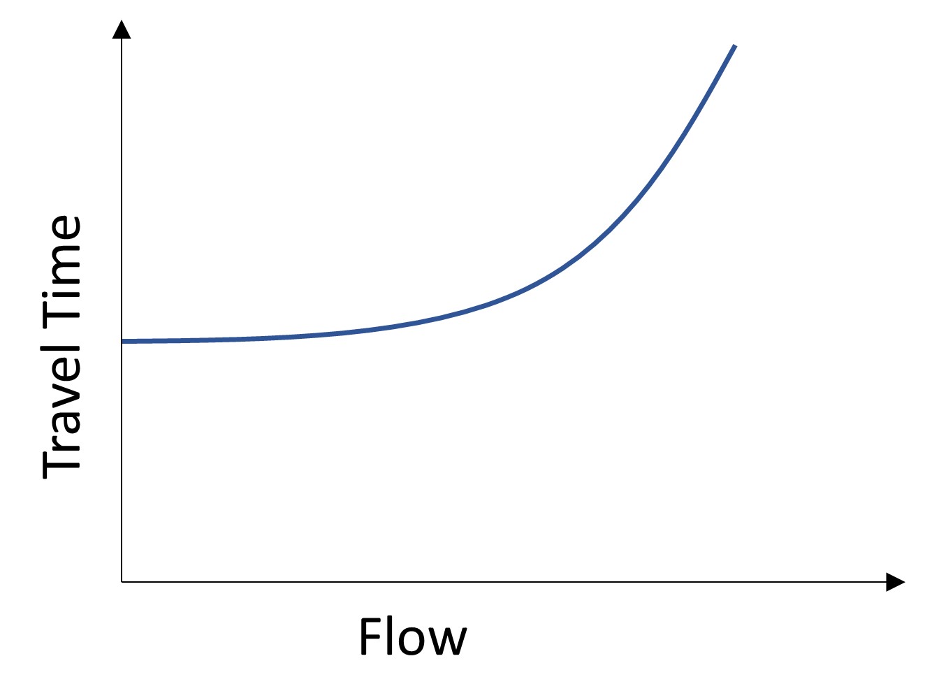
The following example shows how the link performance function helps us to determine the travel time according to flow and capacity.
Performance Function Example
Assume the traffic volume on a path between zone i and j was 525. The travel time recorded on this path is 15 minutes. If the capacity of this path would be 550, then calculate the new travel time for future iteration of the model.
Based on the link performance function, we have:
![]()
Now we have to plug in the numbers into the formula to determine the new travel time:
![]()
Traffic Assignment Models
Typically, traffic assignment is calculated for private cars and transit systems independently. Recall that the impedance function differs for drivers and riders, and thus simulating utility maximization behavior should be approached differently. For public transit assignment, variables such as fare, stop or transfer, waiting time, and trip times define the utility (equilibrium) (Sheffi, 1985). For private car assignment, however, in some cases, the two networks are related when public buses share highways with cars, and congestion can also affect the performance.
Typically, private car traffic assignment models the path choice of trip makers using:
- algorithms like all-or-nothing
- user equilibrium
- system optimum assignment
Of the assignment models listed above, user equilibrium is widely adopted in the U.S. (Meyer, 2016). User equilibrium relies on the premise that travelers aim to minimize their travel costs. This algorithm achieves equilibrium when no user can decrease their travel time or cost by altering their travel path.
- incremental
- capacity-restrained
- iterative feedback loop
- Stochastic user equilibrium assignment
- Dynamic traffic assignment
All-or-nothing Model
Through the all-or-nothing (AON) assignment, it is assumed that the impedance of a road or path between each origin and destination is constant and equal to the free-flow level of service. This means that the traffic time is not affected by the traffic flow on the path. The only logic behind this model is that each traveler uses the shortest path from his or her origin to the destination, and no vehicle is assigned to other paths (Hui, 2014). This method is called the all-or-nothing assignment model and is the simplest one among all assignment models. This method is also called the 0-1 assignment model, and its advantage is its simple procedure and calculation. The assumptions of this method are:
- Congestion does not affect travel time or cost, meaning that no matter how much traffic is loaded on the route, congestion does not take place.
- Since the method assigns one route to any travel between each pair of OD, all travelers traveling from a particular zone to another particular zone choose the same route (Hui, 2014).
To run the AON model, the following process can be followed:
- Step 0: Initialization. Use free flow travel costs Ca=Ca(0), for each link a on the empty network. Ɐ
- Step 1: Path finding. Find the shortest path P for each zonal pair.
- Step 2: Path flows assigning. Assign both passenger trips (hppod) and freight trips (hfpod) in PCEs from zonal o to d to path P.
- Step 3: Link flows computing. Sum the flows on all paths going through a link as total flows of this link.
Example 2 illustrates the above-mentioned process for the AON model
All-or-nothing Example
Table 13.1 shows a trip distribution matrix with 4 zones. Using the travel costs between each pair of them shown in Figure 13.2, assign the traffic to the network. Load the vehicle trips from the trip distribution table shown below using the AON technique. After assigning the traffic, illustrate the links and the traffic volume on each on them.
Table 13.1 Trip Distribution Results.
| From/to | 1 | 2 | 3 | 4 |
|---|---|---|---|---|
| blank cell | Trips Between Zones | |||
| 1 | – | 150 | 100 | 200 |
| 2 | 300 | – | 250 | 100 |
| 3 | 250 | 100 | – | 100 |
| 4 | 250 | 150 | 300 | – |
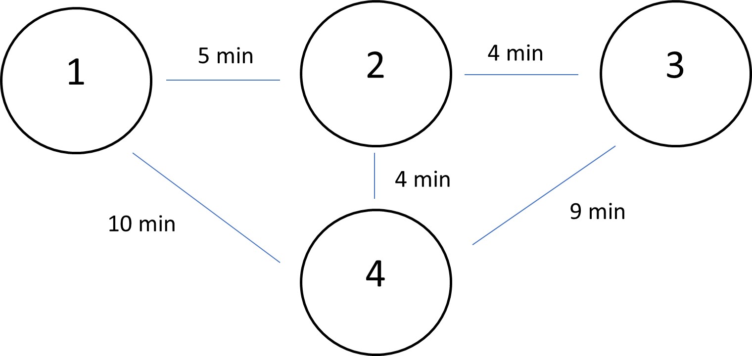
To solve this problem, we need to find the shortest path among all alternatives for each pair of zones. The result of this procedure would be 10 routes in total, each of which bears a specific amount of travels. For instance, the shortest path between zone 1 and 2 is the straight line with 5 min travel time. All other routes like 1 to 4 to 2 or 1 to 4 to 3 to 2 would be empty from travelers going from zone 1 to zone 2. The results are shown in Table 13.2.
| Links | Volume | total |
|---|---|---|
| 1 to 2 | 150+100+200 | 450 |
| 2 to 1 | 300+250+250 | 800 |
| 2 to 3 | 250+250+300 | 800 |
| 3 to2 | 100+250+100 | 450 |
| 1 to 4 | 0 | 0 |
| 4 to 1 | 0 | 0 |
| 2 to 4 | 200+100+100 | 400 |
| 4 to 2 | 250+150+300 | 700 |
| 3 to 4 | 0 | 0 |
| 4 to 3 | 0 | 0 |
As you can see, some of the routes remained unused. This is because in all-or-nothing if a route has longer travel time or higher costs, then it is assumed it would not be used at all.
User Equilibrium
The next method for traffic assignment is called User Equilibrium (UE). The rule or algorithm is adapted from the well-known Wardrop equilibrium (1952) conditions (Correa & Stier-Moses, 2011). In this algorithm, it is assumed that travelers will always choose the shortest path, and equilibrium conditions are realized when no traveler is able to decrease their travel impedance by changing paths (Levinson et al., 2014).
As we discussed, the UE method is based on the first principle of Wardrop: “for each origin- destination (OD) pair, with UE, the travel time on all used paths is equal and less than or equally to the travel time that would be experienced by a single vehicle on any unused path”( Jeihani Koohbanani, 2004, p. 10). The mathematical format of this principle is shown in equation (3):
![]() (2)
(2)
For a given OD pair, the UE condition can be expressed in equation (3):
![]()
![]()
This model assumes that all paths have equal travel time. Additionally, the model includes the following general assumptions:
- The users possess all the knowledge needed about different paths.
- The users have perfect knowledge of the path cost.
- Travel time in a route is subject to change only by the cost flow function of that route.
- Travel times increases as we load travel into the network (Mathew & Rao, 2006).
Hence, the UE assignment comes to an optimization problem that can be formulated using equation (4):
![]() (4)
(4)
Subject to: ![]()
![]()
![]()
![]()
where:
k is the path
xa equilibrium flow in link a
ta travel time on link a
fkrs flow on path connecting OD pairs
qrs trip rate between and
δa,krs is constraint function defined as 1 if link a belongs to path k and 0 otherwise
Example 3 shows how the UE method can be applied for the traffic assignment step. This example is a very simple network consisting of two zones with two possible paths between them.
UE Example
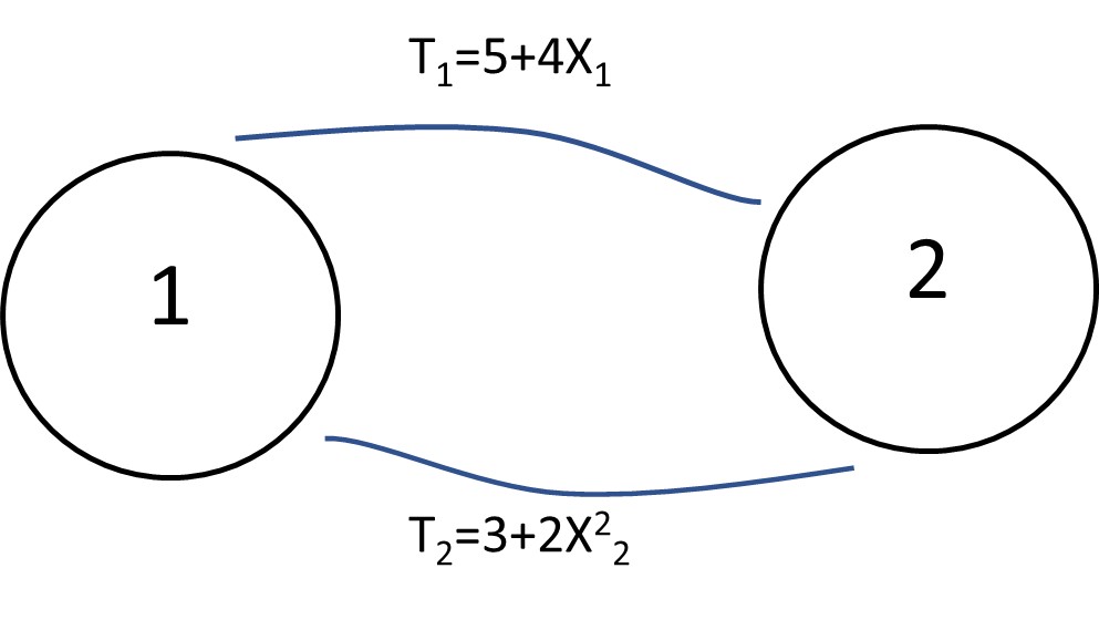
In this example, t1 and t2 are travel times measured by min on each route, and x1 and x2 are traffic flows on each route measured by (Veh/Hour).
Using the UE method, assign 4,500 Veh/Hour to the network and calculate travel time on each route after assignment, traffic volume, and system total travel time.
Solution
According to the information provided, total flow (X1+X2) is equal to 4,500 (4.5).
First, we need to check, with all traffic assigned to one route, whether that route is still the shortest path. Thus we have:
T1(4.5)=23min
T2(0)=3min
if all traffic is assigned to route 2:
T1(0)=3min
T2(4.5)=43.5 min
Step 2: Wardrope equilibrium rule: t1=t2 5+4x1 =3+ 2x22 and we have x1=4.5-x2
Now the equilibrium equation can be written as: 6 + 4(4.5 − x2)=4+ x222
x2 = 2.92
x1 = 4.5 − x2 = 1.58
Now the updated average travel times are: t1=5+4(1.58)=11.3min and T2=3+2(2.92)2=20.05min
Now the total system travel time is:
Z(x)=X1T1(X1)+X2T2(X2)=2920 veh/hr(11.32)+1585 veh/hr(20.05)=33054+31779=64833 min
System Optimum Assignment
One traffic assignment model is similar to the previous one and is called system optimum (SO). The second principle of the Wardrop defines the model’s logic. Based on this principle, drivers’ rationale for choosing a path is to minimize total system costs with one another to minimize total system travel time (Mathew & Rao, 2006). Using the SO traffic assignment, one can solve various problems, such as optimizing the departure time for a single commuting route, minimizing the total travel time from multiple origins to a single destination, or minimizing travel time in stochastic time-dependent O-D flows from several origins to a single destination ( Jeihani & Koohbanani, 2004).
One other traffic assignment model similar to the previous one is called system optimum (SO) in which the second principle of the Wardrop defines the logic of the model. Based on this principle, drivers’ rationale for choosing a path is to minimize total system costs with one another in order to minimize total system travel time (Mathew & Rao, 2006). Using the SO traffic assignment, problems like optimizing departure time for a single commuting route, minimizing total travels from multiple origins to one destination, or minimizing travel time in stochastic time-dependent OD flows from several origins to a single destination can be solved (Jeihani Koohbanani, 2004).
The basic mathematical formula for this model that satisfies the principle of the model is shown in equation (5):
![]()
where:
k is the path
xa equilibrium flow in link a
ta travel time on link a
fkrs flow on path connecting OD pairs
qrs trip rate between and
δa,krs is constraint function defined as 1 if link a belongs to path k and 0 otherwise
Subject to : ![]()
![]()
![]()
![]()
In example 4, we will use the same network we described in the UE example in order to compare the results for the two models.
SO Example
In that simple two-zone network, we had:
T1=5+4X1 T2=3+2X22
Now, based on the principle of the model we have:
Z(x)=x1t1(x1)+x2t2(x2)
Z(x)=x1(5+4x1)+x2(3+2x22)
Z(x)=5x1+4x12+3x2+2x23
From the flow conservation. we have: x1+x2=4.5 x1=4.5-x2
Z(x)=5(4.5-x2)+4(4.5-x2)2+4x2+x23
Z(x)=x32+4x22-27x2+103.5
In order to minimize the above equation, we have to take derivatives and equate it to zero. After doing the calculations, we have:
X2=1.94
X1=2.56
Based on our finding, the system travel time would be:
T1 =5+4*1.94=12.76min T2 =3+ 2(2.56)2=10.52 min
And the total travel time of the system would be:
Z(x)=X1T1(X1)+X2T2(X2)=1940 veh/hr(12.76)+2560 veh/hr(10.52)=24754+26931=51685 min
Incremental Increase model
Incremental increase is based on the logic of the AON model and models a process designed with multiple steps. In each step or level, a fraction of the total traffic volume is assigned, and travel time is calculated based on the allocated traffic volume. Through this incremental addition of traffic, the travel time of each route in step (n) is the updated travel time from the previous step (n-1) (Rojo, 2020).
The steps for the incremental increase traffic assignment model are:
- Finding the shortest path between each pair of O-Ds (Origin Destination).
- Assigning a portion of the trips according to the matrix (usually 40, 30, 20 and 10 percent to the shortest path).
- Updating the travel time after each iteration (each incremental increase).
- Continuing until all trips are assigned.
- Summing the results.
The example below illustrates the implementation process of this method.
A hypothetical network accommodates two zones with three possible links between them. Perform an incremental increase traffic assignment model for assigning 200 trips between the two zones with increments of: 30%, 30%, 20%, 20%. (The capacity is 50 trips.)
Incremental Increase Example
A hypothetical network accommodates two zones with three possible links between them. Perform an incremental increase traffic assignment model for assigning 200 trips between the two zones with increments of: 30%, 30%, 20%, 20%. (The capacity is 50 trips.)
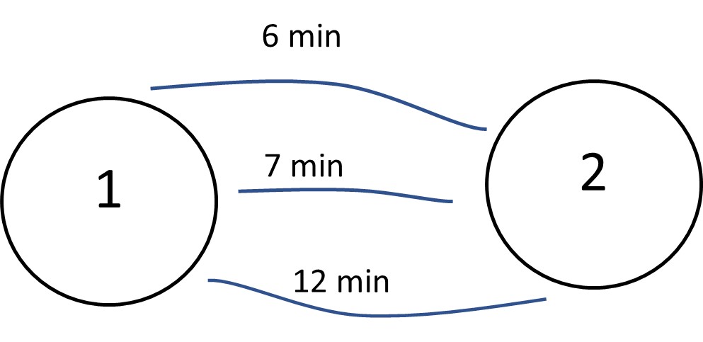
Step 1 (first iteration): Using the method of AON, we now assign the flow to the network using the function below:
![]()
Since the first route has the shortest travel time, the first 30% of the trips will be assigned to route 1. The updated travel time for this path would be:
![]()
And the remaining route will be empty, and thus their travel times are unchanged.
Step 2 (second iteration): Now, we can see that the second route has the shortest travel time, with 30% of the trips being assigned to this route, and the new travel time would be:
![]()
Step 3 (third iteration): In the third step, the 20% of the remaining trips will be assigned to the shortest path, which in this case is the first route again. The updated travel time for this route is:
![]()
Step 4 (fourth iteration): In the last iteration, the remaining 10% would be assigned to first route, and the time is:
![]()
Finally, we can see that route 1 has a total of 140 trips with a 8.85 travel time, the second route has a total of 60 trips with a 9.17 travel time, and the third route was never used.
Capacity Restraint Assignment
So far, all the presented algorithms or rules have considered the model’s link capacity. The flow is assigned to a link based on travel time as the only factor. In this model, after each iteration, the total number of trips is compared with the capacity to observe how much increase in travel time was realized by the added volume. In this model, the iteration stops if the added volume in step (n) does not change the travel time updated in step (n-1). With the incorporation of such a constraint, the cost or performance function would be different from the cost functions discussed in previous algorithms (Mathew & Rao, 2006). Figure 13.5 visualizes the relationship between flow and travel time with a capacity constraint.
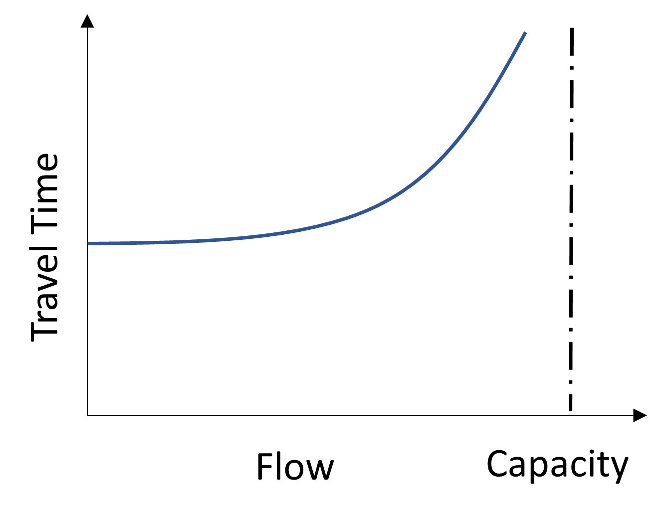
Based on this capacity constraint specific to each link, the α, β can be readjusted for different links such as highways, freeways, and other roads.
Feedback Loop Model (Combined Traffic Assignment and Trip Distribution)
The feedback loop model defines an interaction between the trip distribution route choice step with several iterations. The model allows travelers to change their destination if a route is congested. For example, the feedback loop models that the traveler has a choice of similar destinations, such as shopping malls, in the area. In other words, in a real-world situation, travelers usually simultaneously decide about their travel characteristics (Qasim, 2012).
The chart below shows how the combination of these two modes can take place:
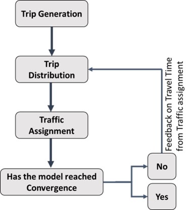
Equation (6), shown below for this model, ensures convergence at the end of the model is:
![]() (6)
(6)
where Ca(t) is the same as previous
Pa is total personal trip flows on link a,
fa is total freight trip flows on link a,
Tod is the total flow from node o to node d,
pod is personal trip from node o to node d,
Fod is freight trip from node o to node d,
ζ is a parameter estimated from empirical data,
K is a parameter depending on the type of gravity model used to calculate Tod , Evans (1976) proved that K’ equals to 1 for distribution using doubly constrained gravity model and it equals to 1 plus attractiveness for distribution using singly constrained model. Florian et al. (1975) ignored K for distribution using a doubly constrained gravity model because it is a constant.
Stochastic User Equilibrium Traffic Assignment
Stochastic user equilibrium traffic assignment is a sophisticated and more realistic model in which the level of uncertainty regarding which link should be used based on a measurement of utility function is introduced. This model performs a discrete choice analysis through a logistic model. Based on the first Wardrop principle, this model assumes that all drivers perceive the costs of traveling in each link identically and choose the route with minimum cost. In stochastic UE, however, the model allows different individuals to have different perceptions about the costs, and thus, they may choose non-minimum cost routes (Mathew & Rao, 2006). In this model, flow is assigned to all links from the beginning, unlike previous models, which is closer to reality. The probability of using each path is calculated with the following logit formula shown in equation (7):
![]() (7)
(7)
where:
Pi is the probability of using path i
Ui is the utility function for path i
In the following, an example of a simple network is presented.
Stochastic User Equilibrium Example
There is a flow of 200 trips between two points and their possible path, each of which has a travel time specified in Figure 13.7.
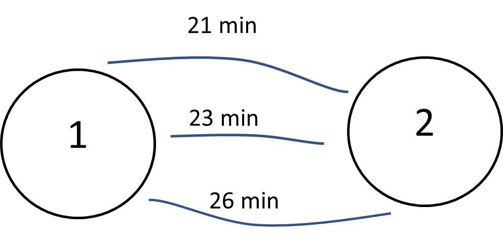
Using the mentioned logit formula for these paths, we have:
![]()
![]()
![]()
Based on the calculated probabilities, the distribution of the traffic flow would be:
Q1=175 trips
Q2=24 trips
Q3=1 trips
Dynamic Traffic Assignment
Recall the first Wardrop principle, in which travelers are believed to choose their routes with the minimum cost. Dynamic traffic assignment is based on the same rule, but the difference is that delays result from congestion. In this way, not only travelers’ route choice affects the network’s level of service, but also the network’s level of service affects travelers’ choice. However, it is not theoretically proven that an equilibrium would result under such conditions (Mathew & Rao, 2006).
Today, various algorithms are developed to solve traffic assignment problems. In any urban transportation system, travelers’ route choice and different links’ level of service have a dynamic feedback loop and affect each other simultaneously. However, a lot of these rules are not present in the models presented here. In real world cases, there can be more than thousands of nodes and links in the network, and therefore more sensitivity to dynamic changes is required for a realistic traffic assignment (Meyer, 2016). Also, the travel demand model applies a linear sequence of the four steps, which is unlike reality. Additionally, travelers may have only a limited knowledge of all possible paths, modes, and opportunities and may not make rational decisions.
Conclusion
In this last chapter of land-use/transportation modeling book, we reviewed the basic concepts and principles of traffic assignment models as the last step in travel demand modeling. Modeling the route choice and other components of travel behavior and demand for transportation proven to be very challenging and can incorporate multiple factors. For instance, going from AON to incremental increase assignment, we factor in the capacity and volume (and resulting delays) relationship in the assignment to make more realistic models. Multiple-time-period assignments for multiple classes, separate specification of facilities like high-occupancy vehicle (HOV) and high-occupancy toll (HOT) lanes; and, independent transit assignment using congested highway travel times to estimate a bus ridership assignment, are some of the new extensions and variation of algorithms that take into account more realities within transportation network. A new prospect in traffic assignment models that adds several capabilities for such efforts is emergence of ITS such as data that can be collected from connected vehicles or autonomous vehicles. Using these data, perceived utility or impedances of different modes or infrastructure from individuals perspective can be modeled accurately, leading to more accurate assignment models, which are crucial planning studies such as growth and land use control efforts, environmental studies, transportation economies, etc.
Glossary
- Route choice is the process of choosing a certain path for a trip from a very large choice sets.
- Regional Transportation Plan is long term planning document for a region’s transportation usually updated every five years.
- Vehicles (VMT) is the aggregate number of miles driven from in an area in particular time of day.
- Total vehicle travel time is the aggregate amount of time spent in transportation usually in minutes.
- Link performance function is function used for estimating travel time, travel cost, and speed on the network based on the relationship between speed and travel flow.
- Hyperbolic function is a function used for linear differential equations like calculating distances and angels in hyperbolic geometry.
- Free-flow road is situation where vehicles can travel with the maximum allowed travel speed.
- Algorithms like all-or-nothing an assignment model where we assume that the impedance of a road or path between each origin and destination is constant and is equal to free-flow level of service, meaning that the traffic time is not affected by the traffic flow on the path.
- Capacity-restrained is a model which takes into account the capacity of a road compared to volume and updates travel times.
- User equilibrium is a traffic assignment model where we assume that travelers will always choose the shortest path and equilibrium condition would be realized when no traveler is able to decrease their travel impedance by changing paths.
- System optimum assignment is an assignment model based on the principle that drivers’ rationale for choosing a path is to minimize total system costs with one another in order to minimize total system travel time.
- Static user-equilibrium assignment algorithm is an iterative traffic assignment process which assumes that travelers chooses the travel path with minimum travel time subject to constraints.
- Iterative feedback loop is a model that iterates between trip distribution and route choice step based on the rational that if a path gets too congested, the travel may alter travel destination.
- First principle of Wardrop is the assumption that for each origin-destination (OD) pair, with UE, the travel time on all used paths is equal and less than or equally to the travel time that would be experienced by a single vehicle on any unused path.
- System optimum (SO) is a condition in trip assignment model where total travel time for the whole area is at a minimum.
- Stochastic time-dependent OD is a modeling framework where generation and distribution of trips are randomly assigned to the area.
- Incremental increase is AON-based model with multiple steps in each of which, a fraction of the total traffic volume is assigned, and travel time is calculated based on the allocated traffic volume.
- Stochastic user equilibrium traffic assignment employs a probability distribution function that controls for uncertainties when drivers compare alternative routes and make decisions.
- Dynamic traffic assignment is a model based on Wardrop first principle in which delays resulted from congestion is incorporated in the algorithm.
Key Takeaways
In this chapter, we covered:
- Traffic assignment is the last step of FSM, and the link cost function is a fundamental concept for traffic assignment.
- Different static and dynamic assignments and how to perform them using a simplistic transportation network.
- Incorporating stochastic decision-making about route choice and how to solve assignment problems with regard to this feature.
Prep/quiz/assessments
- Explain what the link performance function is in trip assignment models and how it is related to link capacity.
- Name a few static and dynamic traffic assignment models and discuss how different their rules or algorithms are.
- How does stochastic decision-making on route choice affect the transportation level of service, and how it is incorporated into traffic assignment problems?
- Name one extension of the all-or-nothing assignment model and explain how this extension improves the model results.
References
Correa, J.R., & Stier-Moses, N.E.(2010).Wardrope equilibria. In J.J. Cochran( Ed.), Wiley encyclopedia of operations research and management science (pp.1–12). Hoboken, NJ: John Wiley & Sons. http://dii.uchile.cl/~jcorrea/papers/Chapters/CS2010.pdf
Hui, C. (2014). Application study of all-or-nothing assignment method for determination of logistic transport route in urban planning. Computer Modelling & New Technologies, 18, 932–937. http://www.cmnt.lv/upload-files/ns_25crt_170vr.pdf
Jeihani Koohbanani, M. (2004). Enhancements to transportation analysis and simulation systems (Unpublished Doctoral dissertation, Virginia Tech). https://vtechworks.lib.vt.edu/bitstream/handle/10919/30092/dissertation-final.pdf?sequence=1&isAllowed=y
Levinson, D., Liu, H., Garrison, W., Hickman, M., Danczyk, A., Corbett, M., & Dixon, K. (2014). Fundamentals of transportation. Wikimedia. https://upload.wikimedia.org/wikipedia/commons/7/79/Fundamentals_of_Transportation.pdf
Mathew, T. V., & Rao, K. K. (2006). Introduction to transportation engineering. Civil engineering–Transportation engineering. IIT Bombay, NPTEL ONLINE, https://www.civil.iitb.ac.in/tvm/2802-latex/demo/tptnEngg.pdf
Meyer, M. D. (2016). Transportation planning handbook. John Wiley & Sons.
Qasim, G. (2015). Travel demand modeling: AL-Amarah city as a case study. [Unpublished Doctoral dissertation , the Engineering College University of Baghdad]
Rojo, M. (2020). Evaluation of traffic assignment models through simulation. Sustainability, 12 (14), 5536. https://doi.org/10.3390/su12145536
Sheffi, Y. (1985). Urban transportation networks: Equilibrium analysis with mathematical programming method. Prentice-Hall. http://web.mit.edu/sheffi/www/selectedMedia/sheffi_urban_trans_networks.pdf
US Bureau of Public Roads. (1964). Traffic assignment manual for application with a large, high speed computer. U.S. Department of Commerce, Bureau of Public Roads, Office of Planning, Urban Planning Division. https://books.google.com/books/about/Traffic_Assignment_Manual_for_Applicatio.html?id=gkNZAAAAMAAJ
Wang, X., & Hofe, R. (2008). Research methods in urban and regional planning. Springer Science & Business Media.
Route choice is the process of choosing a certain path for a trip from a very large choice sets.
Regional Transportation Plan is long term planning document for a region’s transportation usually updated every five years.
Vehicle Miles Traveled (VMT) is the aggregate number of miles driven from an area at a particular time of day.
Polynomial is distribution that involves the non-negative integer powers of a variable.
Hyperbolic function is a function that the uses the variable values as the power to the constant of e.
Hyperbolic function is a function used for linear differential equations like calculating distances and angels in hyperbolic geometry.
Link performance function is function used for estimating travel time, travel cost, and speed on the network based on the relationship between speed and travel flow.
Free-flow road is situation where vehicles can travel with the maximum allowed travel speed.
A point on the curve where the derivation of the function becomes either maximum or minimum.
all-or-nothing is an assignment model where we assume that the impedance of a road or path between each origin and destination is constant and is equal to free-flow level
User equilibrium is a traffic assignment model where we assume that travelers will always choose the shortest path and equilibrium condition would be realized when no traveler is able to decrease their travel impedance by changing paths.
System optimum assignment is an assignment model based on the principle that drivers’ rationale for choosing a path is to minimize total system costs with one another in order to minimize total system travel time.
Incremental model is a model that the predictions or estimates or fed into the model for forecasting incrementally to account for changes that may occur during each increment.
Capacity-restrained is a model which takes into account the capacity of a road compared to volume and updates travel times.
Iterative feedback loop is a model that iterates between trip distribution and route choice step based on the rational that if a path gets too congested, the travel may alter travel destination
Stochastic user equilibrium traffic assignment employs a probability distribution function that controls for uncertainties when drivers compare alternative routes and make decisions.
Dynamic traffic assignment is a model based on Wardrop first principle in which delays resulted from congestion is incorporated in the algorithm.
Wardrop equilibrium is a state in traffic assignment model where are drivers are reluctant to change their path because the average travel time is at a minimum.
First principle of Wardrop is the assumption that for each origin-destination (OD) pair, with UE, the travel time on all used paths is equal and less than or equally to the travel time that would be experienced by a single vehicle on any unused path.
System optimum (SO) is a condition in trip assignment model where total travel time for the whole area is at a minimum.
second principle of the Wardrop is a principle that assumes drivers’ rationale for choosing a path is to minimize total system costs with one another in order to minimize total system travel time
Stochastic time-dependent OD is a modeling framework where generation and distribution of trips are randomly assigned to the area
Incremental increase is AON-based model with multiple steps in each of which, a fraction of the total traffic volume is assigned, and travel time is calculated based on the allocated traffic volume.
feedback loop model is type of dynamic traffic assignment model where an iteration between route choice and traffic assignment step is peformed, based on the assumption that if a particular route gets heavily congested, the travel may change the destination (like another shopping center).
