5 Land-Use and Transportation Modeling I: Land-Use Analysis
Chapter Overview
Chapter 5 delves into various categories of land-use analysis, focusing on the appropriate allocation of land for diverse activities within urban and regional areas. The chapter outlines the steps involved in land-use modeling, dedicating a significant portion to land-use suitability analysis and the essential spatial analysis skills in urban planning. The chapter provides a summary about regional context analysis, community opportunities analysis, demographic and economic interpretation, natural resources and soil analysis, and cultural resources analysis, all of which are important analyses before performing suitability analysis. Next, the chapter introduces the necessary steps to execute these analyses and provides insights into the most commonly employed land-use classifications in practice. In the concluding section, a case study is presented to illustrate the suitability modeling process along with utilizing land-use database sources and mapping techniques.
Learning Objectives
- Understand how to approach land-use modeling step by step and define the important context-based information needed for land-use modeling.
- Describe the general procedure for land-use suitability analysis, and relate it to other planning undertakings and attempts.
- Apply land-use suitability analysis step by step and interpret its results.
- Summarize and compare various land-use classification systems.
- Compare different land-use records to each other using different techniques in GIS environment.
Introduction
In the preceding chapters, we explored how urban areas are shaped by factors like mobility, accessibility, and travel patterns and how the interaction between land use and transportation can alter the spatial structure of cities and regions. This chapter zooms in on a more detailed examination of land-use planning and analysis, presenting the appropriate methods for allocating land within urban and regional areas to accommodate various activities.
Begin with the fundamental question: what activities are occurring where in a city or region? The goal of such queries is the understanding of diverse activity requirements for land and the assessment of whether a piece of land is suitable for a particular activity.
Land use, as defined by Burley (1961), encompasses both land cover and land utilization. Land cover pertains to the surface of the land, including natural elements like vegetation and soil, as well as human-made features such as infrastructure. On the other hand, land utilization refers to the structures, actions, or activities taking place on the land, as explained by Anderson (1976). In practical terms, envision the planning commission in your city deciding to allocate more land to meet the community’s growing needs. This may involve identifying suitable activities for vacant land or redeveloping parcels. The future land-use maps in the municipal comprehensive plan reflect policy decisions, community vision, and input from citizens and stakeholders.
Drawing from various academic works and practices of planning authorities, several analysis techniques are employed to derive recommendations from raw data in land-use analysis. Key primary data for initiating this analysis include:
- the location of the land by a spatial coordination system;
- existing activities on developed land;
- environmental and natural features including surface and subsurface characteristics;
- density of activity on the land;
- ownership information;
- price of the land; and
- existing infrastructure, such as transportation and utility facilities.
Land-use planning and analysis become critical tasks when a community requires additional land and infrastructure for growth. Urban land development involves various stakeholders, including institutional entities, owners, developers, bankers, and local or state governments, each driven by different motives such as market demands, community needs, and the pursuit of a high-quality and sustainable built environment. Considering the influence of these diverse actors is essential when analyzing and making recommendations for land development in urban areas.
Land-use analysis primarily focuses on the current land use, existing development patterns, compliance with federal, state, and local regulations, proposed development patterns, public input, and measurable objectives for implementation (Wang & Hofe, 2020). Land use activities are broadly classified as residential, occupational, or other (non-residential and non-employment). Properly classifying land parcels based on characteristics, location, and intended use ensures effective and efficient land utilization while adhering to relevant regulations or guidelines. In the United States, the externalities of low-density suburban sprawl have heightened pressure on land and resources. Conversely, in developing countries, limited land availability coupled with rapid population growth has accelerated urbanization and development. Recognizing current and past global trends underscores the critical importance of meticulous land-use planning and analysis.
Land-use analysis major considerations
As previously mentioned, the analysis of land-use allocation in an urban setting demands careful consideration of multiple factors. Effectively conducting this analysis involves taking into account various types of data. The following section offers a succinct overview of different techniques intended for analyzing the diverse data types necessary for various levels of spatial analysis. For more in-depth information on the subject, please consult the “Land Use Resource Guide” provided by the Center for Land Use Education at the University of Wisconsin-Stevens Point. For a more detailed exploration of this topic, please refer to the “Land Use Resource Guide” from the Center for Land Use Education at the University of Wisconsin-Stevens Point. This section draws liberally from the Guide’s Chapter 4, “Land Use Analysis,” originally crafted to guide planners in formulating the land use element of a comprehensive plan.
Regional context analysis
Regional context analysis involves identifying and assessing the surroundings of a community. This is crucial because no context exists in isolation, and the surrounding environment significantly influences future land-use development. The regional context encompasses statewide natural features, economic development efforts, transportation locations and decisions, as well as the plans and actions of nearby communities and other agencies (Haines et al., 2005). For instance, economic growth and increased employment in one community can impact housing needs in adjacent areas. Major regional forces affecting a community should always be considered in land-use planning.
Community opportunities analysis
Community opportunities analysis helps in understanding and determining how opportunities influence future land use. The goal is to allocate sufficient land to capitalize on identified opportunities. For instance, in urban areas, it is crucial to identify opportunities that can enhance economic viability downtown or improve the quality of life in neighborhoods, such as implementing waste treatment systems. These opportunities should be prioritized and specified in future land-use plans (Haines et al., 2005).
Demographic and economic data interpretation
The influence of socio-economic factors on future land use is undeniable. Collecting data on population and job trends helps in determining the mutual impact of these developments. To make informed decisions about the future of land-use patterns, it is essential to gather data on factors such as population growth, age levels, workforce size and skills, and economic activities (Haines et al., 2005).
Natural resources and soil analysis
Natural features, conditions, and resources contribute to the character of a community. Including this information in suitability analysis guides decisions about the type and location of development. This analysis should collect information about various kinds of soils, such as agricultural soil and unsuitable soil for development, as well as the location of underground waters, basins, natural preserves, parks, and archaeological sites. Understanding natural and physical barriers to development is crucial. For example, assessing the suitability of soil types for different developments, considering factors like agricultural productivity and load-bearing capacity, provides valuable information for future land-use decisions (Haines et al., 2005).
Cultural resources analysis
Cultural and historical aspects of a community shape a sense of place and guide recommendations for future land-use patterns in accordance with local culture and history. In-depth investigation of local sources of information is necessary to identify cultural heritages requiring special attention and preservation before any land-use change. A key consideration in this analysis is checking whether a resource is listed in the National Register of Historic Places or if a building or site may qualify for the registry (Haines et al., 2005).
Utility analysis
Utility analysis addresses utility system capacities in coordination with future land uses, providing a reliable understanding of existing and future infrastructure and major utility systems, such as sewage or treatment plants. Integrated land-use planning practices assess the amount, density, type, and location of future land uses to coordinate the utility system with the future land-use pattern, ensuring adequate service and protecting the infrastructure from damage or insufficient facilities (Haines et al., 2005).
Transportation system analysis
Transportation system analysis merges land-use planning with the transportation network and the mobility needs of residents and commercial and industrial activities. In addition to considering infrastructure and historical resources, it is important to understand the conditions, capacity, and location of roads adjacent and extended to new developments. Knowledge of transportation plans, such as highway system extensions and regional bike and pedestrian plans, is necessary when suggesting future land uses. Transportation facilities have a direct impact on accessibility, mobility rates, land prices, and density (Haines et al., 2005).
Growth factor analysis
Growth factor estimation helps planners predict factors like population, employment, auto ownership, and travel demand. This analysis assists planners in identifying natural and physical factors affecting how much and where a community may grow in the future. Understanding spatial growth patterns of the past helps identify growth directions, drainage basins, and environmental corridors for sensitive areas, farmlands, or future projects. All these considerations can be mapped as an independent layer in geographic information system software (Haines et al., 2005).
Zoning and build-out analysis
Development regulations, such as zoning and subdivision ordinances, and building codes are crucial for land-use analysis. They provide planners with information about permitted uses, entitlement processes, and development standards, such as setbacks and building height. This analysis may identify areas where future land-use designations conflict with the existing zoning map. Additionally, calculating activity areas at build-out informs future infrastructure needs to meet projected population (Haines et al., 2005).
Land-use demand projections
Demand projections involve identifying how much of each land-use category will be needed in the future. Different techniques and methods are applicable for various land-use classifications, considering their unique characteristics. For example, residential projection involves multiplying dwelling unit demand in the housing component of the municipal comprehensive plan by anticipated average residential densities over the next 20 years. Commercial and industrial land use indicators use current employee density (person per acre) to project total employment over the next 20 years and determine the needed area for commercial land uses (Haines et al., 2005).
Land-use suitability analysis
In this section, we will explore the common approach to land use suitability analysis for various land-use types using criteria classification scores and their respective weights. Urban and regional planners routinely engage in the essential task of evaluating land-use suitability for future developments. The outcomes of this analysis are pivotal for urban planning, management, and the assessment of development proposals. Mapping software, particularly ArcGIS, has been very instrumental in recent years in facilitating this process by evaluating diverse criteria, including environmental, social, and economic factors (Jafari & Zaredar, 2010, (Zone & Zone, 2008a).
The practice of Land-use Suitability Analysis (LSA) is gaining prominence in urban and regional planning. LSA aids in pinpointing the most fitting land use for a specific area, considering its environmental, social, and economic factors. This makes it a valuable tool for promoting sustainable land management. While land suitability assessment extends beyond geographical information systems, many urban planning professionals and scholars regard LSA as a significant contribution of ArcGIS.
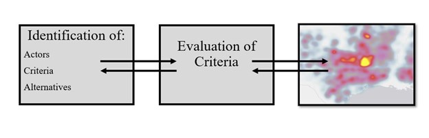
As mentioned earlier, LSA data can encompass various parameters such as soil quality, slope, flood zones, water availability, road classification, accessibility, and activity density. Figure 5.1 illustrates the major steps involved in LSA and the expected results after completing the analysis. The final map, schematically presented on the right-hand side, represents better suitability areas with higher contrasting colors.
To map the suitability of land for different land-use types, a crucial task involves linking various datasets to geospatial locations in ArcGIS. Once completed, the software generates a land-use suitability analysis across different scales and scenarios. Additionally, employing Land Suitability Analysis (LSA) with Geographic Information System (GIS) results in classifying urban and rural areas into zones with varying likelihoods or risks associated with different types of land use.
This mapped information is significant for land-use planning practices. The procedure, grounded in collected and analyzed data, is easy to apply and can be regularly updated (Puntsag et al., 2014).
Given that land-use suitability analysis demands a diverse set of data (criteria) for analysis, transportation data emerges as a crucial component. The integration of LSA with transportation models offers various benefits in the realm of land-use and transportation modeling. Many integrated plans in land use and transportation often begin with an analysis of existing conditions and assumptions about the distribution of future employment, residential areas, and population density.
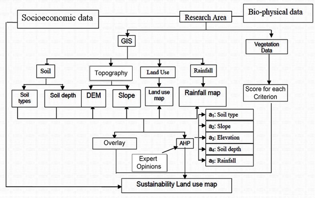
However, by incorporating LSA into land-use transportation modeling, it becomes possible to better identify and map locations for various activities and land uses. In essence, LSA provides socio-economic and demographic projections for the future of the study area (Reibel et al., 2009). Figure 5.2 illustrates the general framework of an LSA for urban service deliveries. Following the preparation of the base map and delineation of the study area, different criteria and variables are mapped and overlaid. Subsequently, using the Analytic Hierarchy Process (AHP) model and expert opinions, each criterion is ranked, leading to the generation of a final score and map.
Steps for land-use suitability analysis
The suitability analysis process involves overlaying maps containing diverse data types, such as physical, locational, and institutional information. The accumulated data results in a score indicating low, medium, or high suitability for a particular development. In Land-Use Suitability Analysis (LSA), the primary assumption is that the suitability score is a linear function of various factors. This method is popular due to its simplicity and appeal to decision-makers and analysts, especially when utilizing GIS (Malczewski, 2004).
According to this method, the suitability of a location (i) for land use (j) can be written as:

Or

where:
S is the ultimate score of a land for a certain land-use type,
F is the suitability of each factor based on their effects for a land I and land use type j, and
b is the coefficient or weight for suitability ratings.
The appropriate rating for different lands and land uses should be based on theoretical knowledge and frameworks that determine the most important affecting variables. As shown, factor weights are also very determining for suitability analysis results, and regression is a common tool for computing these weights. However, many scholars have suggested that when regression analysis is not available, Delphi technique or a multi-criteria evaluation technique, such as Analytical Hierarchy Process (AHP) (Wind & Saaty, 1980) can be implemented. The steps needed to complete the analysis are as follows:
- Step 1: Selecting a land-use category for analysis
- Step 2: Identifying the factors and their assigned values
- Step 3: Determine the score for various attributes for the factors
- Step 4: Weight the factors
- Step 5: Calculate a composite score from attribute value and weight for each factor
- Step 6: Rank the combined scores to establish suitability levels
- Identify the available land based on existing land use
- Constraints with comprehensive plans, zonings, or other land-use controls to further remove unavailable land
Step 1: Selecting a land-use category for analysis
Begin by selecting a specific land-use category for analysis within the Land Suitability Assessment (LSA). This involves examining the suitability of the land for different purposes, such as residential, commercial, or industrial use. In cases where multiple land-use types are proposed for a given area, establish a preference order.
Step 2: Identifying the factors and their assigned values
Identify the factors and their assigned values crucial for the analysis. Choosing these factors is a critical step, as they significantly influence the land’s suitability. Factors encompass diverse data, including the physical state of the land, cost-benefit analysis for the proposed land use, transportation, and utility considerations. It’s important to note that the number and nature of factors vary based on the type of land and its context. Consider local circumstances, available resources, natural hazards, key stakeholders, and residents’ needs to compile a relevant list of factors. For instance, emphasize the importance of accessibility in the analysis, considering factors such as satisfactory access to opportunities, transportation facilities, and utilities (as discussed in Chapter 4). For residential land use, proximity to supporting infrastructure and community facilities is advantageous. Consequently, areas closer to these facilities should be prioritized for development over more remote locations. Analyzing the existing infrastructure network is crucial to include the accessibility factor and assign appropriate values.
Step 3: Determine the score for various attributes for the factors
Proceed by determining the scores for various attributes related to the factors. Attributes may take different data structures, such as nominal, ordinal, interval, or ratio. For example, floodplain data can be nominal (inside or outside the 100-year floodplain), while slope can be measured as a continuous ratio with values between 0 and 90 degrees. To ensure a robust suitability analysis, establish a clear linkage between the suitability score and attributes, ensuring that higher attribute values correspond to a higher level of suitability. Assigning scores may be a challenging task, requiring careful reordering and reclassifying (data cleaning). Refer to Table 5.1 for an example, which illustrates several factors with attributes converted to scores.
| Factor | Attribute | Score |
|---|---|---|
| Slope
|
<5% | 7 |
| 5% 15% | 4 | |
| 15% 25% | 2 | |
| > 25% | 1 | |
| Floodplain
|
Inside 100-year floodplain | 1 |
| Outside 100-year floodplain | 5 | |
| Temperature
|
Slight | 5 |
| Moderate | 3 | |
| Severe | 1 | |
| sensitive natural feature
|
Inside the area | 5 |
| Outside the area | 2 | |
| Distance to major arterials
|
> 1 kilometers | 5 |
| I ~ 2 kilometers | 4 | |
| 2 ~5 kilometers | 3 | |
| > 5 kilometers | 2 |
Step 4: Weigh the factors
In the fourth step of the Land Suitability Assessment (LSA), we focus on determining the significance of the identified factors by assigning weights to each of them. These assigned weights reflect the relative importance of each factor in comparison to others. The weights are typically expressed as percentages, ensuring that the cumulative sum of all factors equals 100%. It’s worth noting that different groups of experts may hold varying opinions regarding the importance and ranking of factors. Similar to step three of the analysis, the Delphi method can be employed in step four. In this method, a group of experts convenes to anonymously provide answers to a series of questions, including numerical value assignments to factors. Through several iterative feedback exchanges, a consensus on the weights can be reached (Grime & Wright, 2016). It’s important to mention that the Delphi method is not limited to step four; it can also be applied to step three. Table 5.2 serves as an example, illustrating weights assigned to five factors identified for assessing the land suitability of residential land use.
| Factor | Weight |
|---|---|
| Slope | 20% |
| Floodplain | 20% |
| Temperature | 10% |
| Sensitive Natural Area | 35% |
| Distance to major arterials | 15% |
Step 5: Calculate a composite score from attribute value and weight for each factor
After identifying the appropriate factors and determining the scores and their weights, it is the time to calculate the composite score using the below formula:

where:
S is the summation of the product of the individual weight,
 is the weight for factor i,
 is the score for each factor.
Step 6 Rank the combined scores to establish suitability levels
After calculating the composite score for the study area, we should rank it based on certain thresholds in order to generate different classifications for land suitability. For instance, a score between 0 and 1 can represent least suitability and a score between 4 and 5 can indicate most suitability. A detailed example of a suitability ranking via scores is shown in table 5.3.
| Composite Score | Suitability Class |
|---|---|
| 0~1 | Least suitable |
| 1.1~2 | Less suitable |
| 2.1~3 | Moderate suitable |
| 3.1~4 | More suitable |
| 4.1~5 | Most suitable |
Step 7: Identify the available land based on existing land use
In the seventh step, the focus is on identifying areas suitable for the proposed land uses. A crucial consideration in this phase is the preference for areas with minimal human impacts and low intensity. This preference stems from the fact that it is generally uncommon to convert land with higher intensity to lower intensity. Consequently, new developments typically occur in undeveloped lands. For instance, farmlands and agricultural areas might be chosen for residential development. After calculating the composite score and comparing it with the characteristics of available lands, the goal is to pinpoint areas with the highest suitability for future developments. This step involves a strategic assessment to ensure that selected lands align with the intended land use and development objectives.
Step 8: Constraints with comprehensive plans, zonings, or other land-use controls to further remove unavailable land
In the final step, proposed developments are reviewed for alignment with municipal comprehensive plans and development regulations. This ensures conformity with environmental conservation areas and considers buffer zones or setbacks, limiting certain land uses and building placements. LSA analyzes ecological and environmental resources, excluding unsuitable areas and prioritizing lands for development within identified suitable zones.
A case study of LSA
The Land Suitability Assessment (LSA) discussed in this section was conducted by Luo Lingjun, He Zong, and Hu Yan in 2008. They utilized remote sensing and GIS technologies, applying the LSA to urban-rural land planning in China. The analysis focused on the Lianping area in China and employed factors derived from land-use interpretation of TM (Thematic Mapper) images. The key factors considered in this analysis included natural limiting factors, economic construction, ecologically sensitive factors, and ecological protection factors. Each of these overarching categories consisted of several sub-factors, which will be elaborated on in the subsequent pages.
The initial step of this study involved identifying and classifying existing land-use types in the Lianping area. This information is crucial as the current land use can act as a significant barrier or motivation for future development. Additionally, the distribution of land uses in the area plays a pivotal role in influencing planned land uses. The classification of lands in this study area encompassed various types, including arable land, woodland, grassland, construction sites, development land, water bodies, and unused lands (Zone & Zone, 2008b). This comprehensive classification laid the foundation for the subsequent steps in the land-use suitability assessment.
Table 5.4 shows the classification of the area’s terrain, one of the most important factors in LSA. The average elevation is 450 meters, and the assignment of scores is based on this value.
The initial step involved identifying and classifying existing land-use types in the Lianping area, such as arable land, woodland, grassland, construction sites, development land, water bodies, and unused lands (Zone & Zone, 2008b). Understanding current land use is crucial, as it influences both barriers and motivations for future development.
Table 5.4 demonstrates the classification of terrain based on elevation, a significant factor in LSA. The scores are assigned according to surface elevation values, with higher scores indicating stronger limitations.
| classification | Extent | score |
|---|---|---|
| unlimited region in terrain | surface elevation between 196and 300meters | 10 |
| weak limited region in terrain | surface elevation between 300and 350meters | 8 |
| general limited region in terrain | surface elevation between 350and 400meters | 5 |
| strong limited region in terrain | surface elevation between 400and 500meters | 3 |
| stronger limited region in terrain | surface elevation more than 500meters or less than 196meters | 1 |
Similar to terrain factors, landscape, proximity to towns, accessibility, proximity to transportation facilities, and ecological sensitivity were selected and assigned scores based on various attributes. The choice of factors depends on the analysis objectives, land development purposes, previous practices, and major characteristics of the study area.
Following factor identification and classification, the next crucial step involved determining the relative weight for each criterion. In this study, the Delphi method, incorporating experts’ consensus on the importance of the factors was employed to calculate weights. The results are presented in Table 5.5.
| Factor description | Weight |
|---|---|
| Ground elevation | 0.2 |
| Slope, aspect | 0.15 |
| Distance from the cities and towns | 0.15 |
| Distance from the main transport network | 0.15 |
| River and reservoirs, woodland, garden, grassland, unused land (including the beach) | 0.2 |
| Basic farmland | 0.15 |
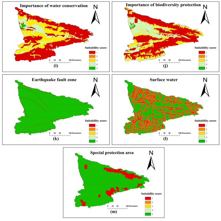
With the factor weights determined, the study employed ArcGIS for spatial data overlay, resulting in visual maps for each factor and an aggregate final score (suitability result), as depicted in Figure 5.3.
Land-use classification
Land-use classification serves as a fundamental data type in Land-Use Suitability Analysis (LSA). It’s aim is to differentiate between various uses and establish appropriate development standards. The roots of land classification trace back to the 1950 report titled “Urban Land Use” by the American Society of Planning Officials. This report documented the profession’s efforts to standardize the mapping and designation of different land uses for analytical purposes. The result was the creation of standardized broad categories of land use, including residential, multifamily, commercial, industrial, railroad, parks, streets, semi-private areas, and more. Since 1950, two major approaches have evolved for classifying land uses: The Standard Land Use Coding Manual (SLUCM) and the Land-Based Classification Standards (LBCS). These coding systems offer greater detail, encompassing additional dimensions of land use, such as typical land use or the type of activity on a parcel, ownership data, density, and structure. Prior to 1950, the firm of Harland Bartholomew & Wood developed a land-use classification applied to the many comprehensive plans that the firm produced for cities across the nation. Land uses were initially categorized into a two-tiered system, where the first level identified the land use category, distinguishing between vacant or developed land, whether private or public. The second level provided details about the type of structures. This approach is straightforward and was later expanded to include ownership data.
| Level 1 | Level 2 |
|---|---|
| Residential
|
Single -family homes |
| Two -family homes | |
| Multiple dwellings (apartments ) | |
| Commercial | |
| Industrial
|
Light industry |
| Heavy industry | |
| Public and Semi -public
|
Schools, churches, hospitals |
| Institutions, golf courses, etc. |
The Standard Land Use Coding Manual (SLUCM) originated in 1965 from a collaboration between the Bureau of Public Roads and the Urban Renewal Administration. This classification system involved four levels of coding, utilizing a 4-digit code to characterize each parcel. Published jointly by the Federal Highway Administration and the Department of Housing, the SLUCM established a comprehensive list of land-use categories with numeric codes based on the Standard Industrial Classification (SIC) system in 1965. It quickly became the nationwide standard for urban land-use coding. Although a reprint was issued in 1972, its usage waned in the late 1970s due to a shift in land-use planning focus towards short-term, small-scale projects, with a reduced emphasis on long-term planning (American Planning Association, 1994). Table 5.7 shows an example of land use classification for residential usage in the City of Dallas, TX. This table is a showing a snapshot of the original table (for the original table follow: City of Dallas Residential Landuse Classification).
| DISTRICT | blank cell | SETBACKS | blank cell | Density | blank cell | Height | Lot Coverage | Special Standard | PRIMARY Uses |
|---|---|---|---|---|---|---|---|---|---|
| blank cell | blank cell | Front | Side/Rear | blank cell | |||||
| A(A) Agricultural |
50′ | 20’/50′ | Dwelling Unit/3 Acres | 24′ | 10% | Agricultural & single family | |||
| R-1ac(A) Single Family |
40′ | 10′ | 1 Dwelling unit/ 1 Acre | 36′ | 40% | Single family | |||
| R-1/2ac(A) Single Family |
40′ | 10′ | Dwelling unit/ 1/2 Acre | 36′ | 40% | Single family | |||
| R-16(A) Single Family |
35′ | 10′ | Dwelling Unit/ 16,000 sq. ft. | 30′ | 40% | Single family | |||
| R-13(A) Single Family |
30′ | 8′ | 1 Dwelling Unit/ 13,000 sq. ft. | 30 | 40% | Single family | |||
| R-10(A) Single Family |
30′ | 6′ | 1 Dwelling unit/ 10,000 sq. ft. | 30′ | 45% | Single family | |||
| R-7.5(A) Single Family |
25′ | 5′ | 1 Dwelling Unit/ 7,500 sq. ft. | 30′ | 45% | Single family | |||
| R-5(A) Single Family |
20′ | 5′ | Dwelling Unit/ 5,000 sq. ft. | 30′ | 45% | Single family | |||
| D(A) Duplex |
25′ | 5′ | 1 Dwelling unit/ 3,000 sq. ft. | 36′ | 605 | Min. Lot: 6,000 sq. ft | Duplex & single family | ||
| TH-1(A) Townhouse |
0′ | 0′ | 6 Dwelling Units/ Acre | 36′ | 60% | Min. Lot: 2,000 sq. ft | Single family | ||
| TH-2(A) Townhouse |
0′ | 0′ | 9 Dwelling Units/ Acre | 36′ | 60% | Min. Lot: 2,000 sq. ft | Single family | ||
| TH-3(A) Townhouse |
0′ | 0′ | 12 Dwelling Units/ Acre | 36′ | 60% | Min. Lot: 2,000 sq. ft | Single family | ||
| CH Clustered Housing | 0′ | 0′ | 18 Dwelling Units/ Acre | 36′ | 60% | Proximity Slope | Multifamily, single family | ||
| MF-I(A) (Multifamily) | 15′ | 15′ | Min lot 3.000 sq. ft. 1,000 sq ft-E 1,400 sq. ft- 1 BR, 1,800 sq ft-2BR | 36′ | 60% | Proximity Slope | Multifamily, duplex, single family | ||
The Land-Based Classification Standards (LBCS), developed by the research department of the American Planning Association in 1994, is likely the most comprehensive land classification system. Serving as an extension of the 1965 SLUCM, this approach features a multi-aspect and multi-scale data structure, encompassing five attributes of land use: activities, functions, building types, site development character, and ownership. However, a 2012 review by the American Planning Association’s research team noted limited adoption of LBCS at the local level. Despite its advantages in specificity and flexibility over single-purpose classification systems, LBCS faces limited deployment. This lack of adoption may stem from a simple lack of awareness among planners (APA, 2012, p. 10). The activity dimension in LBCS pertains to the direct human use of land (American Planning Association, 2009). However, the 2012 review by the American Planning Association’s research team highlights that LBCS adoption at the local level remains limited. Considering its code structure, LBCS could prove beneficial for LSA and integrated land-use transportation modeling.
Table 5.8 displays categories for activity-based classification, illustrating that certain categories can have second-level classifications as well.
| Code | Description |
|---|---|
| 1000 | Residential |
| 2000 | Shopping, business, or trade |
| 2100 | Shopping |
| 2110 | Goods-oriented shopping |
| 2120 | Service-oriented shopping |
| 3000 | Industrial, manufacturing, and waste-related |
Function of the land is the second dimension in this classification system that communicates the economic function or the type of the establishment. In this dimension, each category can be further classified according to different properties of each function. For instance, residence or accommodation functions can include homes, apartments, as well as hotels. Table 5.8 shows some of these functions classifications.
The structure dimension focuses on the establishment’s physical structure on the land, emphasizing the building developed for the land rather than the activity or function. Similar to previous dimensions, structure can be divided into four levels. For instance, in the case of residential buildings, the second level identifies whether the building is for a single-family unit, multi-family unit, or other specialized residential structures. In the next level, it identifies whether the building is detached units, attached units, or manufactured housing. The fourth level includes other properties such as duplexes, zero lot line structures, row houses, etc. (American Planning Association, 2009).
| Code | Description |
|---|---|
| 1000 | Residence or accommodation functions . |
| 2000 | General sales or services |
| 3000 | Manufacturing and wholesale trade |
| 4000 | Transportation, communication, information, and utilities |
| 4100 | Transportation services |
| 4200 | Communications and information |
| 4210 | Publishing |
It is worth noting here that LBSC and SLUCM are two of the widely adopted classification methods used within the context urban planning in the US, although certain cities and regions may develop their own customized version of classification system that is tailored for their specific needs and contextual features. While SLUCM is more focused on land use activities, LBCS has classifications for land cover as well. Additionally, both methods use a hierarchical structure with multiple levels of subcategories, however LBCS is more comprehensive in terms of range of subcategories. Furthermore, it is believed that LBCS can be better customized for specific needs compared to SLUCM and may better integrate with GIS for mapping and analysis purposes. That said, SLUCM is more widely used local government and planning agencies for land use planning, zoning, and development standards, while LBCS is more common for federal agencies and research institutions.
Site development is another dimension in this system that represents data about the physical features of the land. Its three main classes are site in a natural state, developing land, and developed lands. However, for some lands, this dimension might not be applicable. Table 5.9 illustrates this dimension in the LBCS classification system.
| Code | Description |
|---|---|
| 1000 | Site in natural state |
| 2000 | Developing site |
| 3000 | Developed site – crops, grazing, forestry, etc. |
| 4000 | Developed site – no buildings and no structures |
The ownership dimension is the last dimension in the LBCS system, through which the ownership data is classified. The three main general categories in this dimension are: privately owned, public and non-profit sectors, or jointly owned lands. In the following table, various kinds of ownership status are observable. The 2000 category that is labeled as easement restraint refers to a landowner who does not have the sole right of use of the property. Like the previously discussed dimensions discussed here, ownership can also be further categorized into lower levels. For instance, for the lands classified as public restrictions, the next level could be the administrative level of the public owner like state, federal, or even for local government, such as city, village, township, etc.
| Code | Description |
|---|---|
| 1000 | No constraints, private ownership |
| 2000 | Some constraints, easements, or other use restrictions |
| 3000 | Limited restrictions, leased and other tenancy restrictions |
| 4000 | Public restrictions, local, state, and federal ownership |
| 4100 | Local government |
| 4110 | City, village, township, etc. |
| 4120 | County, parish, province, etc. |
| 4200 | State government |
| 4300 | Federal government |
Note. From “LBCS Ownership Dimension with Descriptions” by American Planning Associaton. 2009 (https://www.planning.org/lbcs/standards/ownership/).
5.6 Land databases and mapping
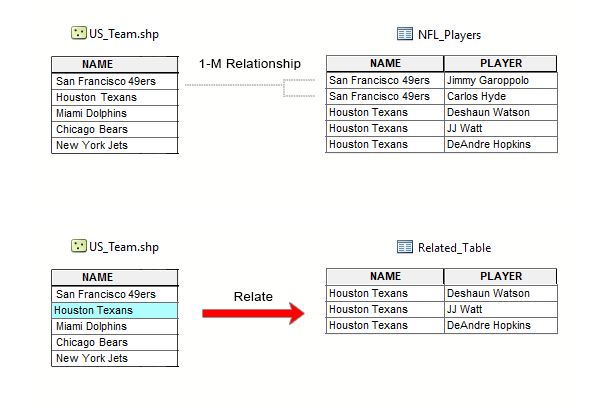
For many years, land data storage was manual, involving the creation of parcel map books. These books, predating the era of computers and digital data storage, assigned a unique Property Identification Number (PIN) to each parcel. Most data, including ownership and land-use type, was recorded using this PIN. Whether in paper-based archives or computerized systems, a common structure for recording land data is a map containing all parcels and associated data with a PIN (Wang & Hofe, 2020). In computerized land-use databases, data tables play a central role. Each row represents a parcel, and each column signifies a variable. An advantageous feature in computerized versions is the ability to join different tables and data using a key field. A key field is a column containing unique values for parcels. There are four types of relationships: one-to-one, many-to-one, one-to-many, and many-to-many. In a one-to-one relationship, one key value in one table matches at most one matching key value in the second table. The connection is typically established using a key variable, often a Feature Identifier Field (FID), appearing only once in each table (Bansal & Pal, 2005). In the many-to-one relationship, the key values in the first table may be duplicated, while the second table maintains unique values. Consequently, records in the first table can be linked to a single key in the second table. Figure 5.4 illustrates a two-step merging of three tables using two key fields related to parcel (tax) information.
One-to-many is a relationship in which the key field in the first table contains unique values and the key field in the second table has duplicated values. In other words, in this joining of tables, we merge one record in the first table to multiple records in the second table.
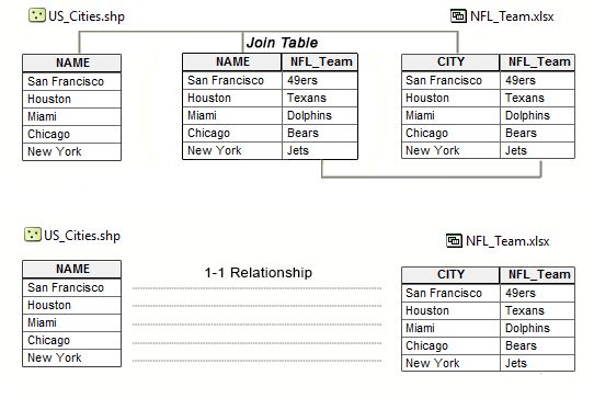
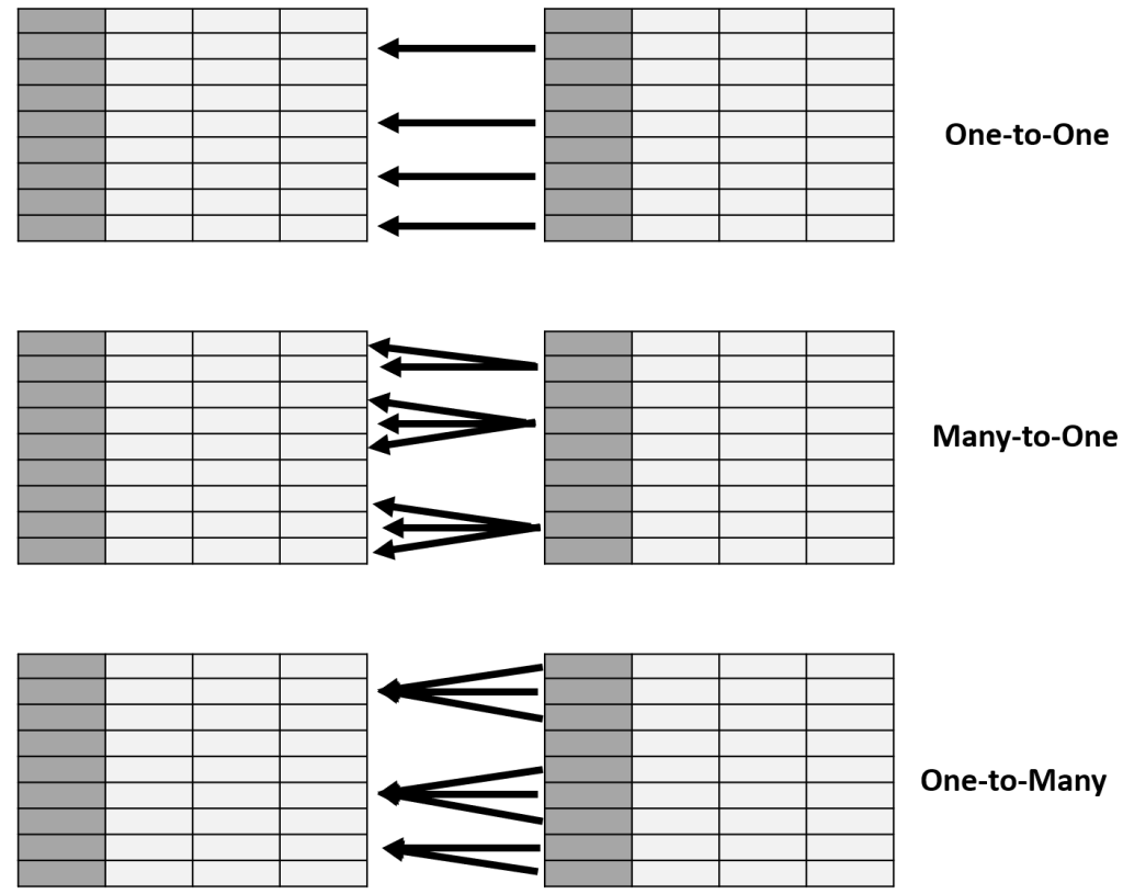
The last type is called many-to-many, where both key fields in the two tables have duplicated values. In this mode, one record in table one can be linked to multiple records in table two and vice versa. For example, we may have various densities within a zip code area, and one particular density may appear in many zip codes. An intermediate table may be needed to connect two tables for this kind of relationship. Figure 5.5 schematically shows how to join different tables using one-to-one, many-to-one, and one-to-many relationships.
Conclusion
In this chapter we reviewed LSA which stands as a powerful and pivotal tool in urban land management. LSA is a multi-step process and this chapter focused on one method for performing LSA. Several other techniques such as index overlay, multi-criteria evaluation, fuzzy logic, machine learning and image classification exists in practice than can utilized depending on local requirements or availability accurate data. As we demonstrated in the case study example, research is still going on to advance techniques of LSA and generate insights for urban planning field. We also reviewed some of the widely-used land use classification systems in the US and highlighted the importance of adoption of such systems for interoperability and reliability of land use data in GIS for planning purposes. With such a rapid rate of urbanization worldwide, and emerging challenges for sustainable development, the usefulness of these evidence-based approaches for informing land use decisions cannot be overstated.
Glossary
- Regional context analysis is a technique for identifying and assessing the surroundings of a community that includes “statewide natural features, economic development efforts, transportation locations and decisions, and the plans and actions of nearby communities and other agencies” (Haines et al., 2005, p.27).
- Community opportunities analysis kind of analysis that helps us to address and decide how opportunities affect future land use.
- Cultural resources analysis type of analysis mainly revolves around the cultural and historical aspects of a community and helps planners to suggest future land-use patterns in accordance to local culture and history
- Utility analysis is an analysis that tries to address the utility system capabilities and their coordination with future land uses
- Transportation system analysis is usually the same as land use and transportation modeling since it is seeking to integrate land-use planning with the transportation network and residents’ mobility needs
- Growth factor analysis is a tool at hand for planners for predicting different factors like population, employment, auto ownership, travel demand, etc
- Land-use suitability is geospatial tool that is used for identifying the most suitable for a particular land use.
- Linear function is a type of relationship between two quantities that forms a straight line with constant slope.
- Delphi technique is structured communication with experts to use their input for decision -making.
- Multi-criteria evaluation technique is a GIS-based tool to identify the most suitable land for a purpose by a multiple criteria.
- Analytical Hierarchy Process is technique for structing the decision making using by quantifying the alternatives and criteria through pairwise comparison to find the best solutions.
- 100-year floodplain is a referred to an area for which the probability of having flood in any given year is 1%.
- Land-use classification is a principal type of data that we need for land-suitability analysis, and we typically base the analysis on the information derived from land-use classification.
- Property identification number a unique number assigned to each parcel by parcel map book which is connected various data like ownership.
- One-to-one is a type of relationship between an object that can relate only to one destination or description.
- Many-to-one is a type of relationship between multiple objects in the first table and one single record in destination table.
- One-to-many is a type of relationship between one object in the first table or layer to many objects in the destination table.
- Many-to-many is when one object in first table can be related to multiple objects in the destination table and vice versa.
- Feature identifier field (FID) a value that is created, assigned and managed by GIS functions to identify a feature or object.
Key Takeaways
In this chapter, we covered:
- Land-use planning and analysis are important tasks in urban planning and development, and various types of data are needed and should be collected for this analysis.
- LSA generally contains eight subsequent steps, by which the most suitable land for a particular land use can be discovered.
- Numerous data records and land-use classifications exist, all of which store certain information about a piece of land such as activity, structure, ownership, etc.
- Four types (techniques) for joining spatial information stored in tables can be used for creating GIS datasets.
Prep/quiz/assessments
- What are the major considerations before starting any land-use development analysis and allocation of lands to activities? Explain any two of them.
- What is the importance of land-use suitability analysis in urban planning and development, and what are general ways to quantify land characteristics?
- What are the steps for land-use suitability analysis and assumptions for creating a suitability score?
- What is the difference between one-to-one, one-to-many, and many-to-one techniques for joining GIS tables?
References
American Planning Association. (1994). Toward a standardized land-use coding standard. Bureau of Public Roads and the Urban Renewal Administration. https://www.planning.org/lbcs/background/scopingpaper/
American Planning Association. (2009). Land-based classification standards. https://planning-org-uploaded-media.s3.amazonaws.com/document/LBCS.pdf
Anderson, J. R. (1976). A land use and land cover classification system for use with remote sensor data (Vol. 964). US Government Printing Office.
Bansal, V. K., & Pal, M. (2005). GIS in construction project information system. In Proceedings of Map India, 8th Annual International Conference and Exhibition in the Field of GIS, GPS, Arial Photography, and Remote Sensing. India https://www.academia.edu/531265/GIS_in_Construction_Project_Information_System
Bartholomew, H., & Wood, J. (1955). Land use in american. Harvard University Press. https://www.amazon.com/Land-American-Cities-Harland-Bartholomew/dp/0674509005
Burley, T. M. (1961). Land use or land utilization? The Professional Geographer, 13(6), 18–20. https://doi.org/10.1111/j.0033-0124.1961.136_18.x
GISGeography. (2022, March 15). Relate vs Join: Cardinality for Attribute Tables in ArcGIS. GIS Geography. https://gisgeography.com/relate-vs-join-attribute-tables-arcgis/
Grime, M. M., & Wright, G. (2016). Delphi method. In P. Brandimarte, B. Everitt, G. Molenberghs, W. Piegorsch, & F. Ruggeri (Eds.), Wiley StatsRef : Statistics Reference Online (pp. 1-6). John Wiley & Sons Inc. https://doi.org/10.1002/9781118445112.stat07879
Haines, A., Walbrun, C., Kemp, S., Roffers, M., Gurney, L., Erickson, M., & Markham, L. (2005). Land use resource guide. Center for Land Use Education, University of Wisconsin-Stevens Point/Extension.
Jafari, S., & Zaredar, N. (2010). Land suitability analysis using multi attribute decision making approach. International Journal of Environmental Science and Development, 441–445. https://doi.org/10.7763/ijesd.2010.v1.85
Joerin, F., Thériault, M., & Musy, A. (2001). Using GIS and outranking multicriteria analysis for land-use suitability assessment. International Journal of Geographical information science, 15(2), 153-174. https://doi.org/10.1080/13658810051030487
Luan, C., Liu, R., & Peng, S. (2021). Land-use suitability assessment for urban development using a GIS-based soft computing approach: A case study of Ili Valley, China. Ecological Indicators, 123, 107333. https://doi.org/10.1016/j.ecolind.2020.107333
Loi, N. K. (2010). Integration of GIS and AHP Techniques for Analyzing Land Use Suitability in Di Linh District, Upstream Dong Nai Watershed, Vietnam. Southeast Asian Regional Center for Graduate Study and Research in Agriculture (SEARCA) (No. 2010-2)
Lingjun, L., Zong, H., & Yan, H. (2008). Study on land use suitability assessment of urban-rural planning based on remote sensing—A case study of Liangping in Chongqing. Remote Sensing Technology and Application, 2008, 23(6): 662-666.https://www.isprs.org/proceedings/xxxvii/congress/8_pdf/1_wg-viii-1/22.pdf
Malczewski, J. (2004). GIS-based land-use suitability analysis: a critical overview. Progress in Planning, 62(1), 3–65. https://doi.org/10.1016/j.progress.2003.09.002
Puntsag, G., Kristjánsdóttir, S., & Ingólfsdóttir, B. (2014). Land suitability analysis for urban and agricultural land using GIS: Case study in Hvita to Hvita, Iceland. United Nations University Land Restoration Training Programme. https://www.grocentre.is/static/gro/publication/434/document/puntsag2014.pdf
Wang, X., & Hofe, R. vom. (2020). Selected methods of planning analysis. Springer Singapore, Imprint Springer.
Wind, Y., & Saaty, T. L. (1980). Marketing applications of the analytic hierarchy process. Management Science, 26(7), 641–658. https://doi.org/10.1287/mnsc.26.7.641
Delphi technique is structured communication with experts to use their input for decision -making.
Multi-criteria evaluation technique is a GIS-based tool to identify the most suitable land for a purpose by a multiple criteria.
Analytical Hierarchy Process is technique for structing the decision making using by quantifying the alternatives and criteria through pairwise comparison to find the best solutions.
100-year floodplain is a referred to an area for which the probability of having flood in any given year is 1%.
Land-use classification is a principal type of data that we need for land-suitability analysis, and we typically base the analysis on the information derived from land-use classification.
Property identification number a unique number assigned to each parcel by parcel map book which is connected various data like ownership.
One-to-one is a type of relationship between an object that can relate only to one destination or description.
Many-to-one is a type of relationship between multiple objects in the first table and one single record in destination table.
One-to-many is a type of relationship between one object in the first table or layer to many objects in the destination table.
Many-to-many is when one object in first table can be related to multiple objects in the destination table and vice versa.
Feature identifier field (FID) a value that is created, assigned and managed by GIS functions to identify a feature or object.
