7 Land-Use and Transportation Modeling III: Southern California Planning Model (SCPM)
Chapter Overview
This chapter elaborates on a specific integrated model, the Southern California Planning Model (SCPM), developed at the University of Southern California in the early 1990s. SCPM is a GIS-based model used for regional planning. Its input-output component reports the results in considerable spatial detail. SCPM modeling framework has been used to estimate and/or forecast economic impacts of activities including terrorist attacks or natural hazards such as hurricanes or flood.
This chapter presents three versions of the SCPM model: SCPM1, SCPM2, and SCPM3. Each model has its assumptions, objectives, methodologies, and applications. Additionally, case studies are used to demonstrate the characteristics and applications of the models. These case studies include examining the economic impact of stormwater treatment technology using SCPM1, estimating the shocks of terrorist attacks on the transportation network and the business interruption losses caused by hurricanes using SCPM2, and modeling the effects of peak-load pricing on passengers and freight using SCPM3.
Learning Objectives
- Identify a new framework for land-use transportation modeling (SCPM) and recognize its significant components.
- Classify and compare the SCPM modeling framework with previous models and summarize its application in urban planning.
- Describe the general process of SCPM and explain the application of economic data (input-output table) in this modeling approach.
- Classify the three versions of the SCPM package based on their unique characteristics and interpret the results from each of them
Introduction
The previous chapters have demonstrated the need to adopt land use and transportation integration modeling approaches for analyzing and simulating future developments of employment centers, residential areas, non-basic economic sectors, and urban transportation network systems. The integration is sometimes more than just land use and transportation. Depending on the specific context, regional economics and infrastructure investments (e.g., transportation and storm water treatment systems) can be incorporated. Another example is the evaluation of the regional economic impact caused by catastrophic events. Models often provide information about the cost of events and the best ways to mitigate them (Cho et al., 2001). This is especially important in today’s policy environment, where U.S. metropolitan areas face multiple challenges, including budget constraints. There is a growing need to measure the impacts of large projects and justify funding decisions on a regional or local scale (Duncan et al., 2012).
Metropolitan areas in the United States are often considered contiguous regions that connect major cities. They are comprised of a network of one or more main cities and surrounding urban areas that are spatially and economically connected in various aspects, including employment, environment, and transportation infrastructure. Further, metropolitan areas accommodate both stationary places and spaces for flows. These flows can be the circulation of information and services with the help of emerging technologies, networks in different specialties, and transportation infrastructures (Lang and Dhavale, 2005).
Modeling and evaluating transportation investments using economic measures aids transportation planning and programming. Refer to OERtransport book, Transportation Planning, Policy and History for more information. Metropolitan Planning Organizations (MPOs) use modeling to comply with performance measures mandated by federal transportation acts, an MPO requirement to qualify for federal funding. Additionally, U.S. highways, bridges, and public transit are often analyzed because of their complexity and numerous impacts on cities and populations. Bridges are often evaluated for their seismic performance.
Modeling bridges is challenging, incorporating complex features such as design and structural performance, and contextual factors like the socio-demographic orientation of the area or severity of natural disasters (Moore, 1999).
As previously mentioned, the development and implementation of modeling for large regions such as US Census-designated combined statistical areas (CSAs) like the Dallas-Fort Worth, TX-OK CSA or the Los Angeles-Long Beach CSA or even megaregions (a group of CSAs) like the Texas Triangle comprising several CSAs is a daunting challenge because of the heterogeneity of data sources for such diverse areas on the one hand and the variety of spatial and temporal definitions on the other. Zonal systems do not capture the functioning of these regions’ boundaries. Political boundaries ignore interrelationships between different ecosystem dynamics (transportation, environment, and socioeconomics) (Pan & Chun, 2020). In these conditions, it is crucial for associations of local governments like the North Central Texas Council of Governments (NCTCOG) or the Southern California Association of Governments (SCAG) to project, analyze, and predict the economic impacts of different projects or events on the region with a detailed spatial dimension.
The Southern California Planning Model (SCPM), the focus ofthis chapter, tries to capture the economic impacts of different infrastructure investments. It may also be used to prepare for unprecedented events in the region. The model incorporates the different scales of zones and jurisdictional boundaries within the region, including the local cities, counties, and subregions. The Southern California Association of Governments (SCAG) website reports that the primary purpose of its integrated land-use transportation models is the ability of the region “to address complex issues and evolving challenges by providing better information about alternative future scenarios and by building an improved linkage between local and regional planning” (SCAG, 2024).
These models utilize regional economic input-output analysis and freight traffic, an urban location model, and transportation network features. The input-output model and its analysis are incorporated into this model because such interaction tables can inform us about the economic structure of the area and the flows of information and freight among industries. Furthermore, the combination of this data and the transportation network can be used to estimate network performance and capacity changes due to economic changes (Moore, 1999).
The Southern California Planning Model (SCPM) is a regional planning model that was developed at the University of Southern California (USC) in the early 1990s to determine the economic impact of different projects and natural disasters (Richardson et al., 1993). This model utilizes a regional input-output model to estimate economic projects’ direct, indirect, and induced effects. The first case study of this model was 219 geographical zones within the five-county region of Los Angeles, which modeled economic outputs and employment flows using a regional input-output model. The SCPM model consists of two major elements which work together to estimate the direct, indirect, and induced effects of different projects. The first main element is an input-output table. This table is a highly disaggregated sectoral model with 494 industries and 93 occupations (a version of the Regional Science Research Institute (RSRI) input-output model). The second element is a spatial allocation of activities using the Garin-Lowry model ( Richardson et al., 1993) , covered in the previous chapter.
SCPM1
In the early 1990s, SPCM was developed to determine the economic impact of different projects and natural disasters (Richardson et al., 1993). The first model utilizes a regional input-output model to estimate economic projects’ direct, indirect, and induced effects. The first case study of this model was 219 geographical zones within the five-county region of Los Angeles in
southern California, which modeled economic outputs and employment flows using a regional input-output model.
The SCPM model consists of two major elements that work together to estimate the direct, indirect, and induced effects of different projects.
- Input-Output table: The first major element is an input-output table presented in Sections 7.2.1 and 7.2.2 below. This table is a highly disaggregated sectoral model with 494 industries and 93 occupations (a version of the Regional Science Research Institute (RSRI) input-output model).
- Spatial allocation of activities: The second element is a spatial allocation of activities using the Garin-Lowry model discussed in Chapter 6, its application to the SPCM1 model is presented below.
SCPM1 Equations
The standard equation for this model is:

where Xi is the total production of commodity of sector i,
Yi is the final demand of commodity of sector i,
Aij is a marginal input coefficient
Additionally, for the matrix formation of the model, the following formula is utilized:

where
X is the production vector
Y is the final demand vector
A is the technical coefficient matrix
7.2.2 Leontief Model Modification
Several limitations of the Leontief input-output model have led to its modification and improvement. For instance, the model excluded households in the initial version and examined goods flow between different industries. The newer version, developed around the 1960s, eliminated this limitation. Another initial feature of this model was its single-region analysis boundary, which means the model assumed that all economic activities and transactions were taking place in a single region. Leontief and Strout (1963) resolved this limitation by developing a framework for multi-region analysis in which each region has both a demand pool and a supply pool. This modification has resulted in minor changes in the model’s underlying equation:

where z denotes the region. Additionally, for projection of interregional flows of commodities, Leontief and Strout (1963) proposed a gravity formula to compute the so-called distribution:

where
Xio,d is the amount of commodity i flowing from region o to region d,
Xi is the total amount of commodity i produced and consumed in all the regions
Kio,d is a parameter estimated from the empirical data
Using this method, Leontief could estimate each region’s interregional commodity flows, total exports, and total imports in the base year and forecast the value for a series of future years in a case study. This model provided a sound theoretical base and directed a viable path to combine economic analysis with transportation modeling to investigate regional freight flows (Pan & Richardson, 2015). In the input-output matrix (I-O), the rows comprised seller data, and the columns comprised buyer data. Households, firms, government, and other agencies can be buyers and sellers.
Several studies have utilized I-O models to assess the economic impact of disasters on a region. This method is relatively simple in terms of data collection and projection. However, the model’s linearity and static nature prevent the modeler from incorporating different constraints, such as price changes, and usually results in overestimation. A critical extension of the model to address uncertainties during these transactions includes scenario analysis, sensitivity tests on parameters, the probability distribution of crucial parameter values, and stochastic simulations. This extension yields a range for estimates rather than point estimates (Richardson et al., 2015).
Garin-Lowry Model
The second element is a spatial allocation of activities using the Garin-Lowry model (Richardson et al., 1993), covered in the previous chapter.
This model estimates direct effects on impacted areas and uses the I-O matrix for estimating indirect and induced effects on zones. The indirect and induced effects based on household expenditures are then distributed spatially throughout the entire region via spatial allocation models. The results from SCPM1 are economic impacts on jobs or dollar values of output by sector and by sub-regional zone. Using a disaggregated approach, this demand-driven model traces economic impacts (intra- and inter-regional) shipments.
In all SCPM models, the input-output model is based on the Regional Science Research Institute (RSRI), which has 494 sectors. The transaction table is adopted from the Bureau of Economic Analysis (BEA). The input-output model can calculate the indirect, induced, and direct impacts. For instance, in a transportation roadway project, the direct impact is reduced household expenditure due to increased tax for this new roadway. This effect can also come from outside the region, and the model can make allowance for such direct impacts. Indirect impacts focus on regional vendors from whom constructors purchase different goods and services, and the induced impacts are only for labor which dollars or jobs can express. Thus, to give a spatial dimension to these calculated impacts, we use the Garin-Lowry model in SCPM1.
In summary, the major components of the model are an input-output model, a journey-to-work matrix, and a journey-to-shop matrix. The journey-to-work matrix helps us track all the commuting flows between residential and work zones and income data. The journey-to-shop or services matrix helps us track retail and personal service purchases.
In SCPM1, journey-to-service is recorded in a matrix by the Southern California Association of Governments (SCAG) as home-to-shop trips along with home-to-other and other-to-other trips. For disaggregation, SCPM1 used the regular political jurisdiction, whereas, in SCPM2 & 3, TAZs are the spatial unit of analysis and will be discussed in the following sections.
In SCPM 1, the beginning point for modeling is the vector of final demands V(d), and total outputs from the open and closed input-output (I-O) models are calculated as follows:


where:
Ao and Ac are matrices of technical coefficients for the open and closed I-O model, and V(o) and V(c’) represent the vectors of output. The notation on c means that the household sector is included. V(c) can be expressed another way and as a sum of three types of outputs which we learned in previous sections (direct (d), indirect (i) and induced (u)).


A similar equation can also be written for the spatial dimension of the model:

where:
Zc is a matrix formation reflecting the impacts disaggregated by both spatial unit and the economic sector. The other three values are described as follows:
Z(d) is the most straightforward value that is exogenous to the model and considered the spatial allocation of the direct outputs.
For Z(i), the allocation of indirect outputs is accomplished by incorporating the proportion of employees in each zone in each sector. We have:
![Z(i)=P. diag[F(i)]](https://uta.pressbooks.pub/app/uploads/quicklatex/quicklatex.com-14875424d19000e06c99b9add53e4250_l3.png "Rendered by QuickLaTeX.com")
where:
P denotes the proportion of employees in each zone, and functions diagonalize the indicated vector.
For the induced impact, we need to trace the households’ expenditure patterns. For this end, the following formula is utilized:
![Z(u)=J^{SH}.J^{HW}.P.diag[F(u)]](https://uta.pressbooks.pub/app/uploads/quicklatex/quicklatex.com-775c2554899894c75c4e1d01f91f677d_l3.png "Rendered by QuickLaTeX.com")
where  and
and  are two matrixes that refer to origin-destination (from services to home and from home to work). The reason for adopting these OD matrixes is that we trace households from home to work & from home to their shopping, services, or personal destinations and then indirectly account for the spatial allocation of the increment of sectoral output satisfying induced household expenditures.
Below, a part of economic sectors for commodity and non-commodity services can be seen in Table 7.1.
| Classification | AGG | USC | Description |
|---|---|---|---|
|
Non-Commodity (Service) Sectors
|
AGG10
|
USC30 | Utility |
| USC33 | Transportation | ||
| USC34 | Portal and Warehousing | ||
| USC36 | Broadcasting and information services | ||
| AGG11 | USC31 | Construction | |
| AGG12 | USC32 | Wholesale trade | |
| AGG13 | USC35 | Retail trade | |
| AGG14 | USC37 | Finance and insurance | |
| AGG15 | USC38 | Real estate and rental and leasing | |
| AGG16 | USC39 | Professional, scientific, and technical services | |
| AGG17 | USC40 | Management of companies and enterprises | |
| USC41 | Administrative support and waste management | ||
| AGG18 | USC42 | Education services | |
| USC43 | Health care and social assistance | ||
| AGG19 | USC44 | Arts, entertainment, and recreation | |
| USC45 | Accommodation and food services | ||
| Classification | AGG | USC | Description |
| Commodity sectors
|
AGG01
|
USC01 | Live animals and live fish & meat, fish, seafood, and their preparations |
| USC02 | Cereal grains & other agricultural products except for animal feed | ||
| USC03 | Animal feed and products of animal origin, n.e.c. | ||
| AGG02
|
USC04 | Milled grain products and preparations, and bakery products | |
| USC05 | Other prepared foodstuffs and fats and oils | ||
| USC06 | Alcoholic beverages | ||
| USC07 | Tobacco products | ||
| AGG03
|
USC08 | Nonmetallic minerals (Monumental or building stone, natural sands, gravel and crushed stone, n.e.c.) | |
| USC09 | Metallic ores and concentrates | ||
| AGG04 | USC10 | Coal and petroleum products (coal and fuel oils, n.e.c.) | |
| USC11 | Basic chemicals | ||
| AGG05 | USC12 | Pharmaceutical products | |
| USC13 | Fertilizers |
SCPM 1 case study
This case study (Moore et al., 2004a) represents the application of the SCPM1 model to assess the economic impacts of implementing water treatment for stormwater in the Los Angeles Area. This study presents nine different cost-analysis scenarios based on different strategies for determining rainfalls, the location of treatment plants, and their size (Moore et al., 2004b).
In this analysis, authors identify three levels of stormwater treatment technologies:
• Level I treatment focuses on settling and removing suspended solids and particulates using screening, grinding and grit removal, influent chemical systems, and primary sedimentations.
• Level II focuses on filtering and disinfecting to remove biological contaminants. Techniques and procedures include primary treatment plus chlorination, dichlorination, effluent filtration, effluent screening, and defoaming. Secondary treatment of stormwater is consistent with beneficial recreational uses.
• Level III (advanced) treatment removes small concentrations of priority toxins and heavy metals. The only standard advanced technique is secondary treatment plus reverse osmosis. Advanced treatment of stormwater eliminates virtually all pollutants and renders it appropriate for beneficial uses such as water for groundwater augmentation.
In this analysis, the authors addressed the following questions:
• Are there alternative treatment plans?
• What would the capital cost estimates for different alternatives be?
• What would each alternative’s annual cost of maintenance and operations be?
• What are the economic impacts of the stormwater treatment plants for the region and its subareas?
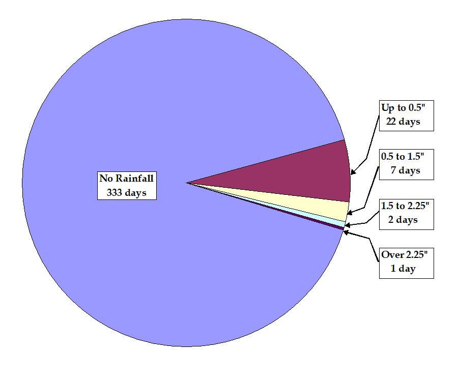
Moreover, the authors created three rainfall scenarios according to Los Angeles County rainfall data. Figure 7.1 shows the number of rainy days with various precipitation rates:
• Scenario I: 1.25 Inches in 24 Hours (Brown & Caldwell, 1998)
• Scenario II: 0.5 Inches in 24 Hours (70% of all wet days)
• Scenario III: 2.25 Inches in 3 days (97% of all wet days)
Finally, three construction cases depending on plant size and their location for each rainfall scenario were developed:
- Case I: 480 plants, 45.2 MG, and 11.1 acres per plant (Brown & Caldwell, 1998).
- Case II: 65 regional plants sited based on geography, one treatment plant per each of Los Angeles County’s sub-basins.
- Case III: 130 plants sited based on political equity, which results in one plant in each city within the area (The total plant numbers would be 132 basin-CDP (Census Designated Places) and 7 residual basins.)
The combination of three rainfall scenarios and three construction scenarios would create a matrix of nine different possible scenarios, each of which has a different economic impact, all analyzed in this study. Next, the authors calculated each scenario’s construction and maintenance costs separately (not elaborated on in this chapter). However, since the total expenditure needed for each combination of scenarios will impact the region’s economy, it was assumed that households in the whole region are taxed for twenty years to repay 4% of 20-year bonds.
Using IMPLAN and SCPM1, IMPLAN outputs were applied to different cities within the five-county southern California metropolitan area. Using the IMPLAN model costs from different scenarios were translated to final regional demand based on the technical coefficients.
According to the results, despite a gain in employment due to construction, more jobs are lost than gained. The range of job losses according to the combination of scenarios is from 20,000 to 150,000. In scenario II for rainfall and construction, 22,000 jobs were lost each year for the first 15 years, and 600,000 in each of the last five years anticipated. It is also possible to translate the impacts from job losses for each sector to dollars. These net values range between 22.649 USD (rainfall scenario II and construction scenario I) to 169.866 USD (rainfall and construction scenario III). Table 7.2 shows the net value losses for the five metropolitan area counties.
| Metropolitan County |
Construction Case I |
Construction Case II | Construction Case III | ||||||
|---|---|---|---|---|---|---|---|---|---|
| Scenario I | Scenario II | Scenario III | Scenario I | Scenario II | Scenario III | Scenario I | Scenario II | Scenario III | |
| Los Angeles | -51,807.7 | -18,267.5 | -98,642.2 | -61,295.3 | -20,022.0 | -125,289.9 | -64,407.3 | -21,191.9 | -136,814.8 |
| Orange | -6,436.8 | -2,272.2 | -12,249.4 | -7,672.6 | -2,504.9 | -15,699.8 | -8,058.2 | -2,652.9 | -17,141.9 |
| Riverside | -1,704.6 | -596.9 | -3,254.3 | -1,971.4 | -645.6 | -4,007.8 | -2,054.0 | -677.5 | -4,323.6 |
| San Bernardino | -2,764.6 | -979.5 | -5,253.2 | -3,336.0 | -1,087.6 | -6,845.7 | -3,518.8 | -1,157.4 | -7,519.1 |
| Ventura | -1,512.5 | -532.4 | -2,878.3 | -1,812.4 | -591.0 | -3,712.6 | -1,908.9 | -628.2 | -4,066.4 |
| Total | -64,226.2 | -22,648.6 | -122,277.5 | -76,087.7 | -24,851.2 | -155,555.8 | -79,947.3 | -26,308.0 | -169,865.9 |
In summary, this study aimed to assess the depressive economic effects of implementing stormwater treatment in nine different scenarios. The stormwater project would need the Los Angeles area and its surrounding jurisdictions to construct, maintain, and operate an extensive network of collection and treatment plants and facilities. The results show that a system that treats stormwater flows from 97% of the region’s annual average storm days will cost about six times more than it would if built to a 70% standard. Also, the stormwater treatment facilities that are financed locally and constructed over 20 years would experience substantial employment and net economic losses (Moore et al., 2004b).
SCPM 2
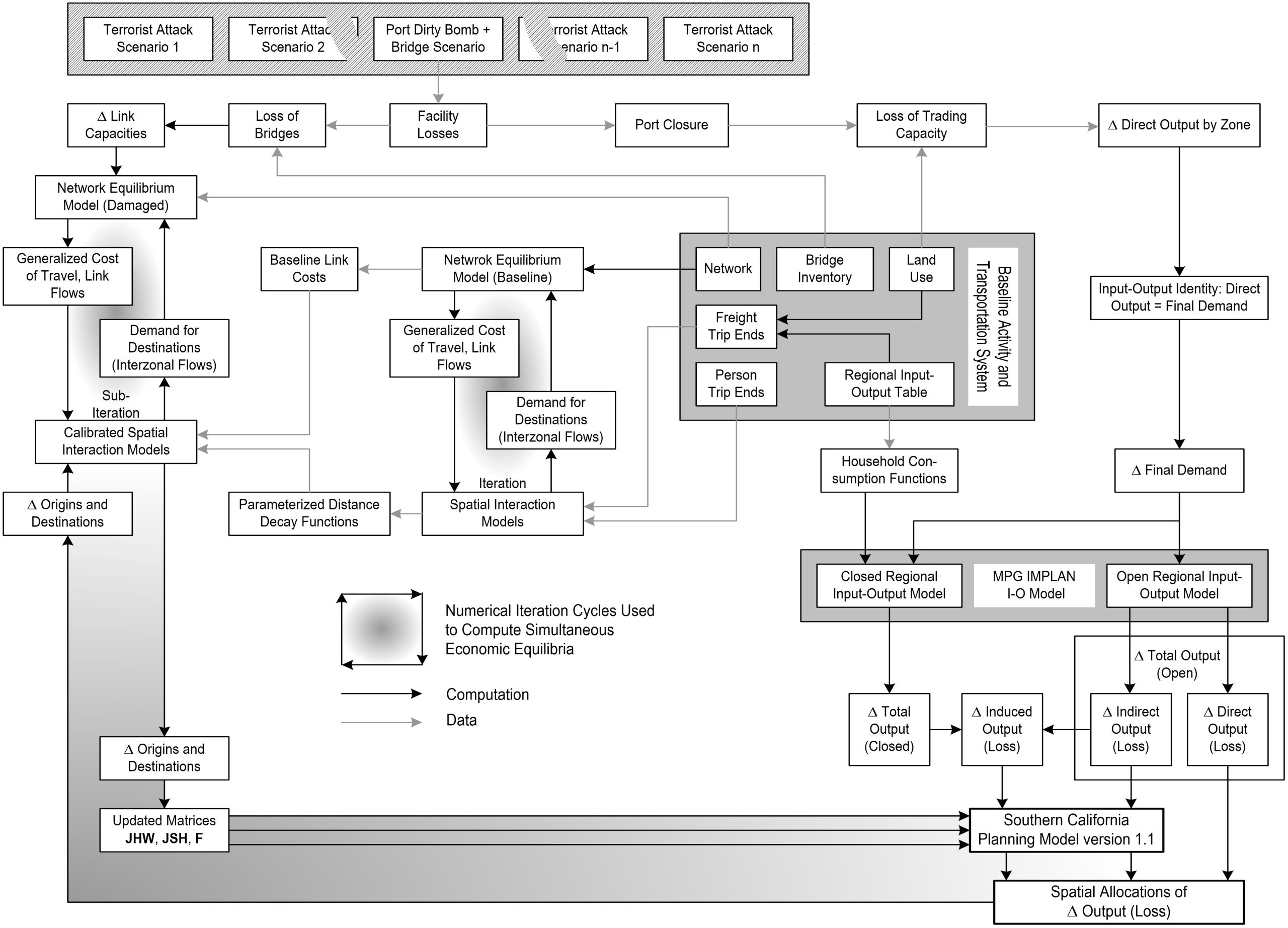
SCPM2 is an advanced modeling process in which traffic flows, such as freight transportation, and the representation of indirect interindustry effects are internalized in the transportation network. Operationalizing the concepts of distance decay and congestion effects is one of the advancements that SCPM2 offers compared to the initial version, SCPM1. This feature permits the endogenization of the spatial allocation of indirect and induced economic losses by route choices and destinations (Sui, 2008). The gravity model illustrates how impacts (determined by the input-output model) affect TAZs. In other words, these economic activities also affect travel behavior and freight movement and reflect how a new equilibrium is achieved. SCPM2 can estimate shipping, infrastructure, and production capacity losses by incorporating the freight databases from regional transportation models. This model’s distribution of traffic flows is only for the AM-peak period for three hours using the static user-equilibrium assignment. The unit of analysis for SCPM2 is the TAZs, aggregated to the level of political jurisdiction. Industry sectors in SCPM2, similar to SCPM1, are reduced to 17 from 515, represented in the Regional Science Research Institute’s PC Input-Output (I-O) model, version 7, based on the work of Stevens et al. (1983). However, more recently, it was disaggregated into 47 sectors, represented in the RSRI database by the IMPLAN I-O model with 509 sectors (Pan, 2015). Figure 7.2 shows the general structure of SCPM2 and its initial application in Southern California. C programming language helped build this model.
Figure 7.2 shows the general structure of SCPM2 and its initial application in Southern California.
C programming language helped build this model. In Figure 7.2, the structure of SCPM1 on the right side is visible, where direct output by zone is generated after losing capacity, and then using the I-O matrix, the indirect and induced effects are calculated. In SCPM2, models on the left represent the cost of travel and commodity flows and are then calibrated based on a new scenario where the capacity of the network is reduced due to the loss of bridges. In turn, the results of this model are used for updating the JHW, JSH, freight matrixes. In this improvement, the distance decay function allows us to endogenize the indirect and induced effects by destination and route choices taking place after reduced capacity (the impact of disaster). Ports and highways act as the backbone of passenger and commodity flows, without them the regular function of a region can be greatly imperiled. Similar to terrorist events, natural disasters such as hurricanes or earthquakes can interrupt such flows. Thus, SCPM2 chose the twin ports of Los Angles as a major hub to estimate economic impacts associated with port closures and bridge losses (Richardson et al., 2015).
SCPM 2 Case Study – Hurricane Effects in Houston, Texas
This section demonstrates the application of SCPM2 in a case study done by Pan (2015) for determining the economic losses due to damages of Hurricane Ike in the Houston Region. The parameters of Hurricane Ike were gathered from the National Hurricane Center (NHC), which Pan (2015) used to estimate the strength of the disaster and its resulting damage at the census tract unit of analysis. To model the spatial allocation of damages and business interruptions, the regional input/output model was used, along with a spatial allocation model, for estimating various damages in the Greater Houston Region. This study develops a general framework that helps estimate losses from actual disasters, direct effects (business interruption losses), total indirect and induced business interruption losses, and their allocation to small analysis zones. This study’s model (SCPM2) also includes trip origin-destination matrices to allocate induced impacts.
Before going over the details of the case study, we must understand how to calculate different effects (direct, indirect, and induced). Business interruption in a hurricane is the most serious direct effect of the disaster. Building recovery time (BRT) and employment information can help us calculate the direct effects using the following formula:
![\mathrm{L}_{\mathrm{z,s}}\mathrm{=}\mathrm{J}_{\mathrm{zs}}\mathrm{*}\left[\mathrm{\sum}_\mathrm{d}\mathrm{} \left({\mathrm{DS}}_{\mathrm{zs,d}}\mathrm{*} {\mathrm{BRT}}_{\mathrm{s,d}}\mathrm{*} \mathrm{F}_{\mathrm{s,d}}\right)\right]](https://uta.pressbooks.pub/app/uploads/quicklatex/quicklatex.com-95fb63048a9192252fce167190ca8acd_l3.png "Rendered by QuickLaTeX.com")
where:
Lzs = total job losses · day in industrial sector s in zone z
Jzs = Number of jobs in each sector (s) and zone (z)
DSzs,d = probabilitiy of damage states in damage state (d), occupancy class (or sector) s, and
zone z;
BRTs,d = Recovery time (borth clean-up and reconstruction or repair) measured as days in damage state (d)
Fs,d = multipliers for building and/or service interruption time
The next step in economic loss modeling is determining the indirect effects. One standard approach to this end is to employ regional I-O models to calculate indirect and induced effects from the direct final demand. Indirect effects here are calculated by the following formula in which employment weighted attractions and productions by sector by zone are incorporated:

where:
IndirS,Z =Total indirect effects in sector (s) and zone (z);
IndirectsS =total indirect effects in sector s; and
ES,Z = Total number of jobs in sector s in zone z.
For induced effects, the usual approach is to allocate the impacts using the O-D matrix in two categories: (1) journey home-to-work origin-destination (O-D) matrix, and (2) a journey home-to- shop O-D matrix. However, not all the cases have available data on these trips, and the alternative is to relate induced effects to impact zones based on damage states of residential buildings, assuming that impact analysis zones are able to accommodate all the home-to-shop trips of residents living in zone (z).

![Rdmg_t = \sum_{1} RInv_{s,s} \ast \left[ \sum_{d} \left( DS_{s,\omega d} \ast BRT_{s,d} \ast F_{s,s} \right) \right]](https://uta.pressbooks.pub/app/uploads/quicklatex/quicklatex.com-52e73b04cc758cd24f9572a0322d8459_l3.png "Rendered by QuickLaTeX.com")
where:
Indurs,z = induced effects in zone z and industrial sector s;
Induceds = total induced effects in sector s in the region;
Rdmgz = Damage occurred to residential building in zone z; or total damage on residential buildings (number of damaged buildings * recovery days) in zone z; and
RInvz,s = Residential building inventory in zone z with occupancy class (s).
The following chart shows the general framework used for estimating losses from real natural disasters:
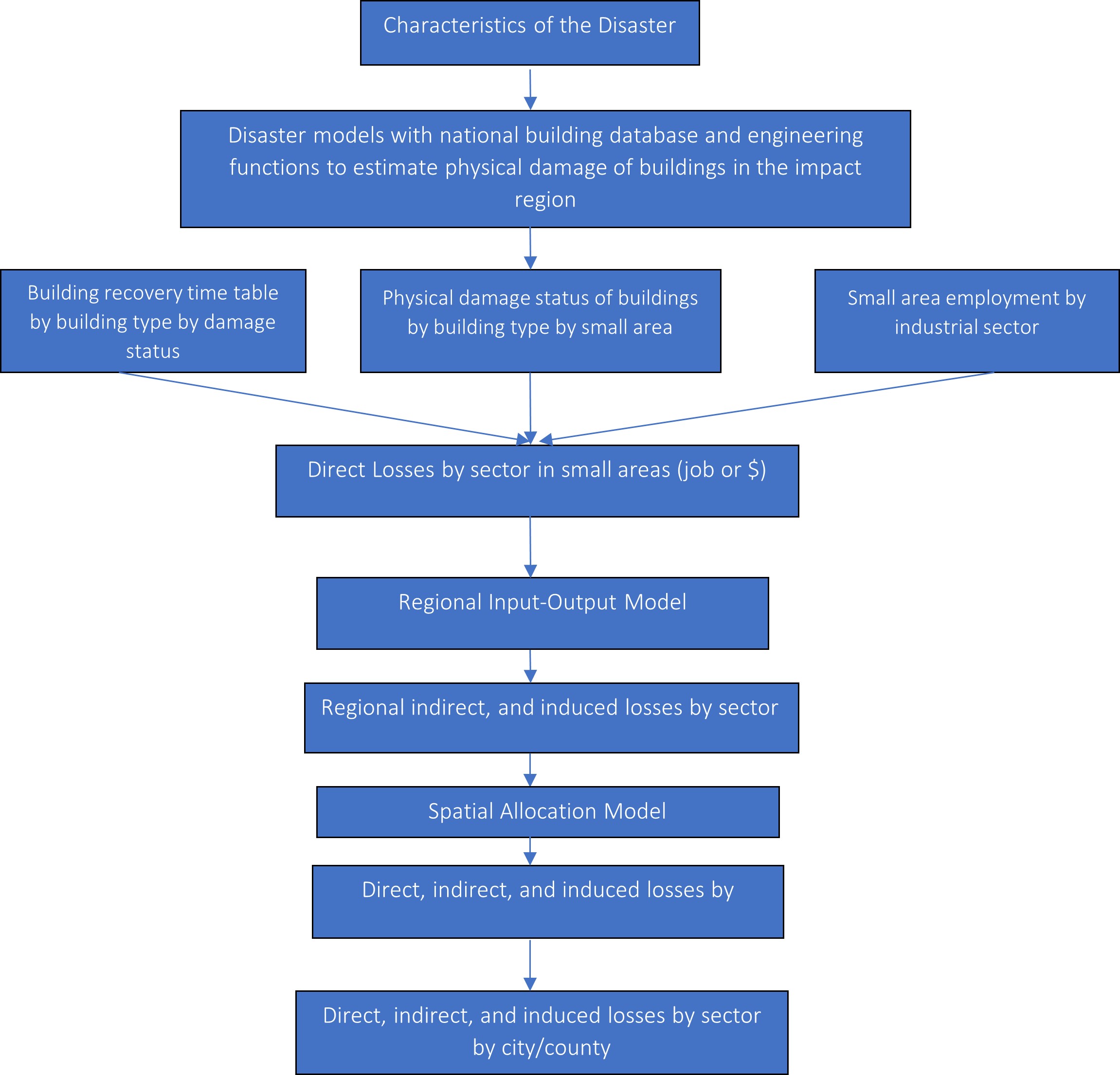
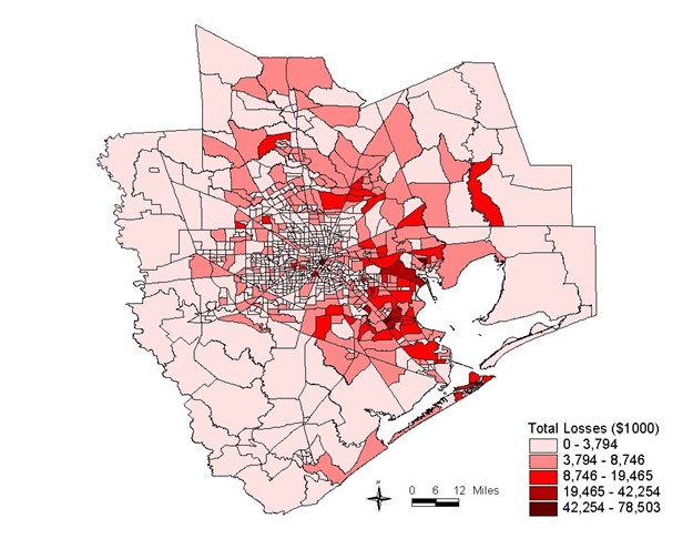
With a general understanding of the approaches and formulas for calculating different kinds of effects, we will continue discussing the case of Hurricane Ike and its economic impacts on the Houston Region. As the first step, the hurricane characteristics should be known. This information includes latitude, longitude, translation speed, radius to max winds, radius types, wind speed, and central pressure. Additionally, the observation unit in this study is 866 census tracts of the Houston Region. The preliminary results of the model estimation were $20.6 billion of property damage and $3.9 billion of income-related business interruption losses. The Hazards-United States (HAZUS) model manual helped estimate building interruption times and their multipliers. Employment data came from the InfoUSA business database, which helps derive standard industrial codes and the number of jobs for each code (sector). The direct, indirect, and induced effects were calculated according to the process and utilizing the formulas presented above. The job losses are converted to dollar value losses using an I-O transaction table. The following map shows the spatial allocation of total loss in the study area (Pan, 2015).
SCPM 3
In the SCPM2 version, we saw how freight transportation (transportation network) is incorporated into the SCPM model using the I-O matrix data. We explored how applying this newly added feature to SCPM can determine the indirect and induced effects of economic activity using the distance decay & gravity model concept. To spatially estimate economic impacts throughout all TAZs, the innovation of SCPM3 is the introduction of the time-of-day choice. In other words, SCPM3 is a more transportation-oriented model by which we can model movement patterns for freight and passengers at various times of the day. Typically, different time periods during the day are aggregated as follows:
- AM peak (6-9 AM),
- PM peak (3-7 PM), and
- Off-peak traffic (9 AM-3 PM and 7 PM-6 AM).
The input for this version again consists of an I-O matrix from a regional input-output model, employment data by TAZ, O-D matrix, freight O-D matrix, regional transportation network dataset, and official political/jurisdictional boundaries. The transportation network data for this study came from SCAG for the year 2000 regional transportation model. This model also incorporates highways’ entry-exit points as external zones. The initial application of SCPM3 was to estimate and understand the effects of peak-loading pricing on a complex land-use-transportation system, including the impacts on transportation network performance (level of service) at the link level and the impacts on activities at a TAZ level (Gordon, Pan, & Center, 2011).
SCPM3 Equations
For traffic assignment to the transportation network, this model applies user equilibrium with variable demand (UE-VD), where the level of service of the network influences trip rates. For instance, users may change the time of their trip (departure); thus, the model incorporates the time-of-day concept.
The formulation of (UE-VD) according to Sheffi (1985) is as follows:

Subject to 


where
xa is the total flow on link a;
ta(x) is the cost function for measuring average travel costs on link a
ϭ oda,p is link-path incidence variable;
h oda,pis the flow (traffic count) connecting origin (O) and destination (D);
Tod is peak-hour trips between origin (O) and destination (D);
 is the total trip between origin (O) and destination (D); p is the link between O and D; and
D -1o,d is the inverse of the demand function for O-D pair (o,d).
The demand function in this model uses a logit formula that addresses the change of demand in congestion time. The function can be written as:

where:
to,d refers to the minimum travel time at peak-time between O and D;
to,d is the minimum travel time at free flow period between O-D pair;
To,d refers to the total trips allocated for peak period using trips-in-motion factors between O-D pair; and
θ is a parameter that should be calibrated locally based on previous data, or a value should be assigned based on local knowledge.
Then the inverse demand function would be:

Additionally, the link cost-flow function can be written as:
![t_a=t_a(0)\left[1+\lambda\left(\frac{x_a}{K_a}\right)^\beta\right]](https://uta.pressbooks.pub/app/uploads/quicklatex/quicklatex.com-423fe562c73e3f237ac2082a5783a424_l3.png "Rendered by QuickLaTeX.com")
where ta(x) is the cost-flow function to calculate the average travel cost on link a, and ta(0) is the free-flow travel cost on link a;
Xa is the aggregate flow of both passenger and freight on link a, including both personal trips and freight trips;
Ka is the capacity of link a; and
α and β are model parameters that need calibrations, while 1+ α is the ratio of travel time per unit distance at capacity Da, and both parameters are estimated from empirical data. In most of the studies, these values are assigned to 0.15 for α and 4 for β (Gordon, Pan, & Center, 2011).
The solution algorithm is summarized as follows:
Step 0: Initialization: At the beginning, we perform an all-or-nothing (AON) traffic assignment model based on free flow travel cost on the network and obtain a feasible solution from the model.
Step 1: Update: According to Step 0, we must update the travel time using the inverse demand function.
Step 2: Find a feasible descent direction: Updated travel times would be used for another AON assignment, providing the modeler with auxiliary link flows.
Use the updated travel time {ta} for an all-or-nothing trip assignment. It yields a set of auxiliary link flows.
Step 3: Find optimal parameter: A linear approximation algorithm (LPA), such as the golden-section method, is applied to obtain the optimal parameter satisfying the UE-VD equation.
Step 4: Update link flows: Link flows (counts) and O-D flows (counts) are updated.
Step 5: Test Convergence: A convergence condition should be observed where link flows are optimal, and an equilibrium condition is reached. Otherwise, we must repeat the process from Step 1.
SCPM 3 Case Study – Modeling of Effects of Peak Load Pricing on Metropolitan Network and Activities
As mentioned earlier, the initial application of SCPM3, developed by Pan et al. (2011), was to model the impacts of peak-load pricing on the major thoroughfares in the five-county Los Angeles Metropolitan Area. Since the model incorporates the time-of-day choice, the fixed demand assumption for each time in this model is relaxed.
Peak-load congestion pricing is regarded as a technique to compensate for the transportation externalities such as air pollution or congestion pricing. This technique motivates travelers to switch their trips out of the peak hours. To realize these travelers’ decisions, we must understand how the users perceive the trade-off between money and time. The appropriate questions for this goal are:
- How should we approach flow modeling between different locations multiple times of the day?
- What would the change in network level-of-service and urban development effects of deploying this policy be?
The data sources for this modeling attempt are the same as discussed in this section. This model incorporates both passenger and freight transportation. However, the difference between freight and passenger travel behavior is that freight is usually affected by a toll on changing routes but not by the time of day to travel.
This study initially assumed two scenarios with two different pricing schemes: a $0.3 per mile and a
$0.01 per mile for two (AM and PM) peak periods, and these tolls were applied to all freeway links in both mentioned times. Moreover, the time costs of peak-load congestion were converted to hours per mile based on the data on hourly wages estimated from IMPLAN 2001. Accordingly, the $0.01 pricing scenario yielded 0.0057 hr/mile, and the $0.03 pricing scenario yielded 0.017 hr/mile. Incorporating these values in the formulas and algorithms described earlier, the results were able to answer the following:
How would various toll scenarios improve levels of service in the area? Which pricing policy is best for a trade-off choice between changing travel time, paying more, or traveling less? What would the
revenue implications of each scenario be? What would the implications of each scenario in terms of urban development in the area be?
| Time period | Road type | $0.30 per mile toll | $0.10 per mile toll | ||
|---|---|---|---|---|---|
| % Change of total travel time | %Change of average travel time | % Change of total travel time | % Change of average travel time | ||
| AM peak | Highway | -54.16% | 50.15% | -13.17% | -14.15% |
| AM peak | Local | 43.08% | 55.61% | 12.31% | 11.03% |
| AM peak | Total | 2.73% | 11.72% | 1.74% | 0.58% |
| PM peak | Highway | -56.55% | 54.18% | -15.18% | -15.78% |
| PM peak | Local | 51.28% | 59.53% | 12.85% | 12.04% |
| PM peak | Total | 7.95% | 13.84% | 1.59% | 0.86% |
| Off-peak | Highway | 8.29% | 2.83% | -1.15% | -0.40% |
| Off-peak | Local | 7.02% | 1.63% | -1.00% | -0.25% |
| Off-peak | Total | 7.53% | 2.11% | -1.06% | -0.31% |
| Daily | 6.50% | 6.95% | 0.41% | 0.34% | |
The results revealed that drivers show substantially different behavior in terms of using tolled or non-tolled roads depending on the pricing scenarios.
As a result, assuming 250 workdays each year, the annual revenue from the lower price scenario generates far more revenue than the higher price scenario. The higher pricing scenario can transfer peak-load traffic to off-peak hours. In contrast, the lower pricing scenario had only minor effects in these terms. Also, an improvement in the level of service for tolled roads comes at the expense of increasing demand for non-tolled roads. The results show that the aggregate travel time increases in the higher pricing scenario since most riders try to avoid the toll. Thus, a great trade-off lies ahead for policymakers – better internalization of transportation externalities, improved transportation level of service, or more revenues collected from tolls (Pan et al., 2011).
Conclusion
In this chapter, the SCPM modeling framework was detailed and its application in different research areas and purposes was demonstrated using three different case studies. From a resiliency perspective and the need for responsive urban systems and planning processes, it is needed to develop frameworks that utilizes standard frameworks to estimate economic gains or losses as result of new projects, developments, or hazardous events such as flooding or terrorist attacks. Furthermore, it is important to estimate the spatial extents of these impacts for multiple purposes such as insurance estimations or planning issues like equity or environment. For instance, using these frameworks we can estimate the total loss imposed on marginalized groups vs normal populations and derive analytics that show how vulnerable different groups of population might be in catastrophic events. SCPM offers a strong model that is based on large-scale and aggregate urban models, became viable after advancements in computational capacities. Although SCPM highly disaggregate economic sectors, its representation of households behavior still suffer from aggregation problems and may not depict the complete picture. Availability of accurate input-output table for economy of Metropolitan areas is another challenge due to openness of economic boundaries of such regions.
Glossary
- Southern California Planning Model (SCPM) is a regional planning model that was developed at the University of Southern California (USC) in the early 1990s to determine the economic impact of different projects and natural disasters and utilizes a regional input-output model to estimate economic projects.
- Contiguous regions or megaregions are a network of one or more main cities and surrounding urban areas spatially and economically connected in different aspects such as environment, employment, and transportation infrastructure.
- Transportation network is a system or graph of corridors distributed in space that permits movement of people and goods.
- Marginal input coefficient is the change in input divided by change in output in I-O matrix.
- Technical coefficient matrix is an element in the input-output model which is the collection of input-output coefficients.
- Linearity is the condition of establishing linear relationships between quantities.
- Scenario analysis is strategic method for planning and decision making that involves defining and evaluating a number alternative for a goal.
- Sensitivity tests is test for determining the uncertainty in the output of a model and the share of each input in that uncertainty.
- Probability distribution is a distribution that shows the probability of occurrence of an incident in an experiment.
- Stochastic simulation is a type of simulation where probabilities for change in variables is inserted in the model through randomization.
- Distance decay is the decline in the number of trips with increasing distance.
- the static user-equilibrium assignment is a assignment model of traffic into network assuming that each user chooses the shortest path for their travel.
- Spatial allocation model is a model that uses the amount of activities in an area as an input and predicts the distribution of industries, employment, population and travel demand.
- Cost-flow function is function that calculates the average travel cost on a link, using capacity and free-flow cost.
Key Takeaways
In this chapter, we covered:
- To model the direct, indirect, and induced effects of events or policy scenarios using the SCPM model.
- To incorporate economic data with land-use and transportation data for prediction purposes of urban development.
- Explored the characteristics of three SCPM versions
- Explored the data required for building and modeling three types of SCM models and looked at their applications.
Prep/quiz/assessments
- What three types of impacts result from different events, such as natural disasters? Moreover, how can each of them be measured?
- What are the two significant elements of the SCPM1 modeling framework? Describe.
- What is the main difference between SCPM1 and SCPM2? Furthermore, what additional results can SCPM2 generate compared to SCPM1?
- What is the data required for the SCPM3 model? Moreover, what is the initial traffic assignment model of SCPM3?
References
Cho, Sungbin, Peter Gordon, James E. Moore II, Harry W. Richardson, Masanobu Shinozuka, and Stephanie Chang. 2001. “Integrating transportation network and regional economic models to estimate the costs of a large urban earthquake.” Journal of Regional Science 41 (1): 39–65. https://doi.org/10.1111/0022-4146.00206.
Duncan, Chandler, Steven Landau, Derek Cutler, Brian Alstadt, and Lisa Petraglia. 2012. “Integrating transportation and economic models to sssess Impact of infrastructure investment.” Transportation Research Record 2297 (1): 145–53. https://doi.org/10.3141/2297-18.
Federal Highway Administration (US) and Federal Transit Administration (US). 2017. 2015 Status of the Nation’s Highways, Bridges, and Transit Conditions and Performance Report to Congress. Government Printing Office.
Gordon, P., & Pan, Q. (2011). Towards peak pricing in metropolitan areas : modeling network and activity impacts. (METRANS Transportation Center (Calif.), Ed.). ROSA P. https://rosap.ntl.bts.gov/view/dot/23271
Lang, R., & Dhavale, D. (2005). Beyond megalopolis: Exploring America’s new “Megapolitan” geography. Brookings Mountain West Publications, 1–33. https://digitalscholarship.unlv.edu/brookings_pubs/38
Moore, J. E., Kuprenas, J., Lee, J. J., Gordon, P., Richardson, H., & Pan, Q. (2004). Cost analysis methodology for advanced treatment of stormwater: The Los Angeles Case. Journal of Construction Research, 5(02), 149-170. https://doi.org/10.1142/S1609945104000127.
MOORE, J. I. (1999). Integrating transportation and economic models. In Technical Council on Lifeline Earthquake Engineering Monograph No. 16, Proc. of the 5th US Conference on Lifeline Earthquake Engineering, American Society of Civil Engineers, Reston, Virginia, 1999 (pp. 621-633).
Input-Output Tables (IOTs) – OECD. (2022.). Www.oecd.org. https://www.oecd.org/sti/ind/input-outputtables.html
Pan, Qisheng. 2015. “Estimating the economic losses of hurricane Ike in the Greater Houston Region.” Natural Hazards Review 16 (1): 05014003. https://doi.org/10.1061/(ASCE)NH.1527-6996.0000146.
Pan, Q., & Chun, B. (2020). Develop a GIS-based Megaregion Transportation Planning Model (University of Texas at Austin. Cooperative Mobility for Competitive Megaregions, Ed.). ROSA P. https://rosap.ntl.bts.gov/view/dot/58659
Pan, Q., Gordon, P., Moore, J. E., & Richardson, H. W. (2011). Modeling of effects of peak load pricing on metropolitan network and activities. Transportation Research Record. https://doi.org/10.3141/2255-02
Pan, Q., Richardson, H.W. (2015). Theory and methodologies: Input–Output, SCPM and CGE. In: Richardson, H., Pan, Q., Park, J., Moore II, J. (eds) Regional economic impacts of terrorist attacks, natural disasters and metropolitan policies. advances in spatial science. Springer, Cham. https://doi.org/10.1007/978-3-319-14322-4_2
Richardson, H W, P Gordon, M-J Jun, and M H Kim. (1993). “PRIDE and prejudice: The economic impacts of growth controls in Pasadena.” Environment and Planning A: Economy and Space 25 (7): 987–1002. https://doi.org/10.1068/a250987.
Richardson, H. W., Pan, Q., PakC., & Moore, J. E. (2015). Regional economic impacts of terrorist attacks, natural disasters and metropolitan policies. Springer.
Sheffi, Y. (1985). Urban transportation networks (Vol. 6). Prentice-Hall, Englewood Cliffs, NJ.
Stevens, B. H., Treyz, G. I., Ehrlich, D. J., & Bower, J. R. (1983). A new technique for the construction of non-survey regional input-output models. International Regional Science Review, 8(3), 271-286.
Sui, D., & Springerlink (2008). Geospatial technologies and homeland security : Research frontiers and future challenges. Springer. Netherlands.
Contiguous regions or megaregions are a network of one or more main cities and surrounding urban areas spatially and economically connected in different aspects such as environment, employment, and transportation infrastructure.
term for a combination of adjacent metropolitan (MSA) and micropolitan statistical areas (µSA) across the 50 U.S. states and the territory of Puerto Rico that can demonstrate economic or social linkage
Megaregions are generally regions that contains two or more adjacent metropolitan areas that have continuous interactions in terms of transport, economy, resources and ecology.
Transportation network is a system or graph of corridors distributed in space that permits movement of people and goods.
Marginal input coefficient is the change in input divided by change in output in I-O matrix.
Technical coefficient matrix is an element in the input-output model which is the collection of input-output coefficients.
Linearity is the condition of establishing linear relationships between quantities.
Scenario analysis is strategic method for planning and decision making that involves defining and evaluating a number alternative for a goal.
Sensitivity tests is test for determining the uncertainty in the output of a model and the share of each input in that uncertainty.
Probability distribution is a distribution that shows the probability of occurrence of an incident in an experiment.
Stochastic simulation is a type of simulation where probabilities for change in variables is inserted in the model through randomization.
O-D trip matrix is a matrix in four step travel demand model that shows the flows of trips between each pair of zones.
Spatial allocation model is a model that uses the amount of activities in an area as an input and predicts the distribution of industries, employment, population and travel demand.
Cost-flow function is function that calculates the average travel cost on a link, using capacity and free-flow cost.
