Land-Use and Transportation Modeling IV: MEPLAN, TRANUS, TELUM, and PECAS

Qisheng Pan; Soheil Sharifi

8 Land-Use and Transportation Modeling IV: MEPLAN, TRANUS, TELUM, and PECAS

Chapter Overview

Chapter 8 concludes the discussion of integrated land-use transportation modeling and describes the features and applications of four popular models. The first model introduced is known as MEPLAN and uses a mathematical framework to model the spatial economies of cities or regions. The second model is known as TRANUS, which simulates activities across space. Different land uses and real estate markets move through the various spatial scales of the transportation system, such as cities, metropolitan areas, regions, and nations. The third one is known as TELUM, a predictive model and software package evaluating the land-use impacts of transportation projects and forecasting the spatial location of employment and households. The last model presented is the Production, Exchange, and Consumption Allocation System (PECAS), which exerts a spatial input-output and econometric model to allocate goods, services, and labor through flows between different locations in an urban area. In this chapter, the framework, model sub-modules, and steps to apply the models are unpacked.

Learning Objectives

Explain the general structure of MEPLAN and its modeling goals, recognize its modules, and relate them to the modeling goals.
Describe the framework of the TRANUS model and summarize the procedure within each sub model.
Explain the application of the TELUM model, categorize different data required by the model, and interpret the model’s outputs.
Explain the application of the PECAS Model, its two sub-models, and the relationship between them.

Introduction

The application of integratedlanduse/transportationmodels has increased over the past decades. Hensher (2004) states that more than 20 contemporary urban land-use transport models exist. Thesemodels are integrated and comprehensive toforecast the need and location of urban land uses, such as residential, public service,industrial,oragricultural(Hensher,2004).

As presented in detail in Chapter 6, Lowry (1964) first attempted to model the feedback between land use and transportation by combining an equilibrium model that incorporated residential, manufacturing, and service sectors. The Lowry model and its successors rely on random utility models for predicting spatial choice behavior. Random utility theory (aka discrete choice theory) tries to forecast the behavior of different actors, such as investors, households, firms, and travelers, in the spatial formation of cities. Through these models, the choice between alternatives, each with a particular set of attributes, is predicted based on stochastic distributions of some events controlling for unobservable attributes of alternatives. These alternatives may stem from differences in people’s preferences, decision-making processes, developers’ inclinations, or a lack of reliable information (Domencich & McFadden, 1975). The approach for such forecasting typically uses multinomial logit models. (Hensher, 2004).

This chapter briefly presents four models – MEPLAN, TRANUS, TELUM, and PECAS – for incorporating land market data, featuring endogenous prices, and facilitating market clearing at each step whereas TELUM is specifically designed for transportation considerations.

The foundational framework of these models relies on export base theory, as elucidated by Li (2015), to establish links between population dynamics and non-basic employment with exogenously projected forecasts of export industries. Employing discrete choice modeling, these three models intricately divide the urban region into subareas and temporally segment activities into discrete time periods. Spatial input-output matrices serve as the bedrock for data in these models, facilitating the projection of goods flows. Intersectoral flows are determined by input-output coefficients or demand functions.

To enhance the spatial dimension of the models, a random utility approach, proposed by Hensher (2004), is used because it captures nuanced preferences and choices, making the models even more sophisticated. Essentially, the models presented in this chapter offer a comprehensive approach to understanding and predicting the complex interplay of transportation, activity location, and market dynamics within urban regions. In the following sections, we will examine each model, highlighting their unique features and contributions to the field.

MEPLAN

In the beginning, three closely related land-use/transport interaction models were developed for three cities – Bilbao (Spain), Dortmund (Germany), and Leeds (England) – by the firm, Marcial, Echenique & Partners. The model software package is known as MEPLAN (Echenique et al., 1990).
MEPLAN is a modeling system consisting of three sub-modules: 1) space allocation sub-modules, 2) transportation sub-modules, and 3) interaction sub-modules.
MEPLAN focuses on analyzing a region’s spatial economy by explicitly incorporating the interaction between land use and transportation within each city zone. It calculates the equilibrium price of land or buildings by considering the demand from various land use activities and the available supply. Additionally, the model assesses the equilibrium price for transportation, factoring in aspects like time and convenience.
Another crucial aspect of the model involves examining the interaction between the travel demand and the transportation supply.
The third key component of the model involves capturing the feedback loop between land use and transportation, particularly in response to changes in accessibility. This feedback loop influences the equilibrium price for land and the spatial distribution of activities, as highlighted by Echenique et al. in 1990. The model’s outcomes yield a set of trip matrices distributed across the transportation network, considering constraints on transportation network capacity and considering multi-modality.
These trip matrices incorporate travel times, which, in turn, determine the disutilities associated with different locations. Ultimately, these disutilities play a crucial role in shaping the location choices for various activities within the region.

In the MEPLAN process for a given timeframe, the sequence begins with running the land market model, followed by the transport market model. Subsequently, an incremental model is employed to integrate feedback between these two components. The interactions, such as updated travel times, from a specific time are introduced into the model as new inputs. For instance, the rise in transportation costs during one period becomes information fed into the land-use model in the subsequent period. This iterative approach enhances the model’s responsiveness to alterations in the location preferences of land uses in reaction to changes in transportation conditions (Abraham & Hunt, 1998).

MEPLAN Modules

The land market in this model is a spatially disaggregated matrix or an input-output table containing technical coefficients and categories of activities, land use, or types of buildings (Abraham & Hunt, 1998). Activities are distributed into the zones by employing a logit model based on zone attractiveness, such as manufacturing costs, locational utilities, and transportation costs of goods.

Figure 8.1 illustrates the primary components (modules) of the model and the dynamic interactions between them, presented in a feedback loop format over time.

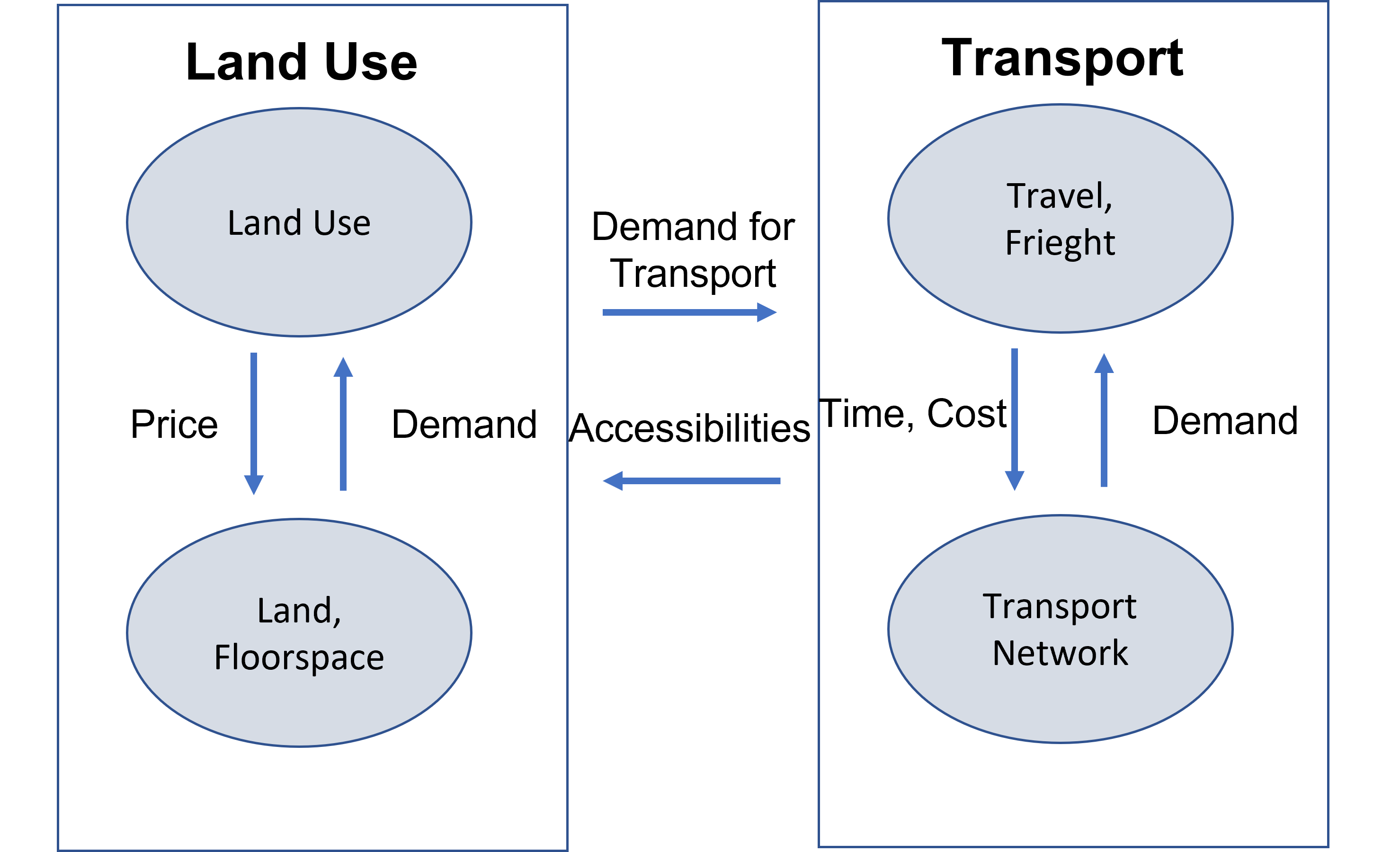
Connection of transport/land use by locational accessibility and transportation demand. — **Figure 8.1** Connection between land use and transportation in MEPLAN models. From “The MEPLAN models of Bilbao, Leeds and Dortmund Foreign summaries,” by M. Echenique, A. D. J. Flowerdew, J. D. Hunt, T. R. Mayo, I. J. Skidmore & D. C. Simmonds, 2007, *Transport Reviews, 10(4),* p. 310. Copyright 2007 by Taylor & Francis Group.

MEPLAN is a modeling system that utilizes entities, such as households or employment locations, to compute housing units or floor space across the various sectors zones in the city. It carefully considers the interdependence of activities, recognizing that each unit of output relies on inputs from other activities, employees, and available floor space. The Input-Output (I-O) matrix captures the interconnectedness between diverse activities. Additionally, each activity is spatially defined, and inputs like labor and services can be acquired from any zone based on selling prices and transportation costs.

The model establishes links between households and firms, conducting multiple iterations through all chains of demands for inputs to generate outputs and determine the locations for obtaining these inputs. The model attains equilibrium or convergence when there are no further changes in activity locations or input prices between iterations.

Once equilibrium is reached, the model determines the actual personal trips (i.e., work, shop, etc.) and freight movement. The model then performs a modal split and a multi-path probabilistic model, accounting for capacity restraints to complete the traffic assignment. The land use modeling part incorporates the results from this part, including updated travel times and costs, to generate new locations and activity demand.

Based on the explanation provided above, we can identify five distinct modules within the MEPLAN package:

Land Use Module (LUS): This module attempts to predict the location of economic activities. This module represents the spatial economic linkages between activities and finds the locational equilibrium point.
Interface Module (FRED): This module’s task is to transform the results produced by the previous module, such as trading patterns or transactions, into personal trips or goods. It can also reverse, transforming the transport disutilities into impedances for trading between different activities.
Transport Module (TAS): This module performs a four-step transportation model according to the flow type and reaches a satisfactory level of convergence employing the transport network features as input.
Evaluation Module (EVAL): This module compares different scenarios, one for testing a particular policy and one for doing nothing. This module can estimate economic efficiency, like cost-benefit analysis.
Graphics Option (GRAPH): This module allows the graphical representation of the generated results as maps, charts, and network plots.

MEPLAN Strengths and Limitations

MEPLAN possesses several notable strengths. Its flexibility lies in the use of logit models, ensuring that the output is easily interpretable. The utilization of an Input-Output (I-O) matrix enhances its suitability for regional analysis. The comprehensive nature of MEPLAN is attributed to the inclusion of various actors within its framework. Lastly, the iterative nature of the model allows for the observation of changes over time, incorporating valuable feedback.

The equilibrium model has limitations due to market failures in various sectors, such as housing or labor (vacancy rates and unemployment). It can only consider past variables for future decisions. This presents a significant drawback, as it overlooks the potential for agents to adjust decisions based on anticipated trends rather than relying solely on historical data. Therefore, a limitation of MEPLAN is its inability to facilitate decision-making based on near future trends or events. Since the incremental model cannot simultaneously solve variables in the current time, it is crucial to choose an appropriate time or sequence for the model to generate accurate and stable results. (Abraham & Eng, 1998).

TRANUS

TRANUS is another integrated land-use/transportation modeling package that combines activity allocation with a transportation model. Similar to the previously mentioned model, TRANUS utilizes the framework of random utility or discrete choice for modeling and simulation purposes (Briassoulis, 2019). The TRANUS software package was developed by Modelistica in Venezuela from a lab by Dr. Toman de la Barra in 1982. TRANUS has been adopted across many regions in the U.S., including Maryland, Sacramento, and Baltimore, and worldwide (Hunt et al., 2005).

TRANUS is applicable for predictions and estimations for a wide range of urban scales, from regions, metropolitan areas, and regions, to states, and provinces, to national-level analysis and even international regions consisting of several countries. Moreover, the range of subjects or topics for which TRANUS can be used is also vast. Implications of land use policies are also predictable by TRANUS since the policy change directly affects the demand and supply of land. Congestion, level of service, development plans, zoning controls, housing projects, housing incentives, environmental plans, road construction, road improvement, public transit planning, tolls, HOV (High Occupancy Vehicle) lanes, congestion pricing, parking pricing, and land use relocations are all among the projects and policies that can be modeled in TRANUS.

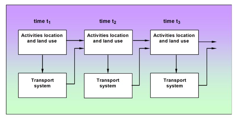
Since all the predictions in these models (like housing location, transportation mode, and firm location) are discrete rather than continuous, random utility theory is an appropriate choice for modeling since this theory helps predict the probability of an occurrence given the input features. Figure 8.2 shows a schematic representation of TRANUS. In this figure, a dynamic interaction between land use and transportation has been devised for different periods, and a full package for activity allocation and transportation separately for each period. In the following section, we discuss the land use or activity allocation and transport models and their interaction.

Flowchart of iterative process of TRANUS model, from activity locations and travel demand. — **Figure 8.2** TRANUS Modeling Framework. From Analysis of Land Use Change: Theoretical and Modeling Analysis of Land Use Change: Theoretical and Modeling Approaches, by H. Briassoulis, 2000, Web book of Regional Science. In the public domain.

In this figure, a dynamic interaction between land use and transportation has been devised for different periods, and a full package for activity allocation and transportation separately for each period. In the following section, we discuss the land use or activity allocation model, the transport model, and their interaction.

TRANUS Sub-models

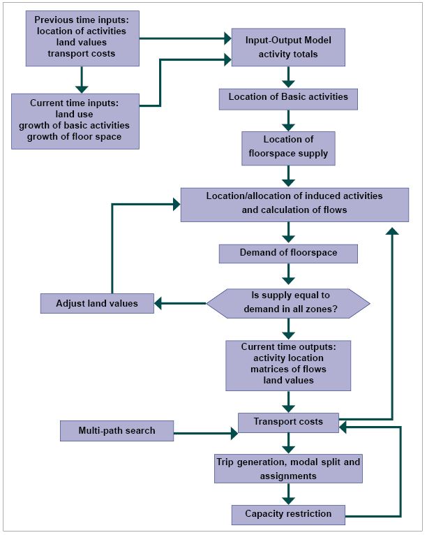
Like the previous models, TRANUS employs the I-O matrix and derives a set of technical coefficients with an aspatial dimension. In this sub-model, we replace the commodities and economic sectors with activities (refer to the number of workers or residents). The activity allocation sub-model relies on two crucial inputs. First, it considers the activities, land values, and transportation costs in each zone within the urban area from previous periods, treated as exogenous factors. Second, for the current time inputs, the model considers land use, the growth of basic activities, and floor space growth.

The first step is to calculate the total induced employment given the exogenous information regarding basic employment. It is also essential to calculate and consider the increment of basic employment and floor space for the current period for each zone. A simple probabilistic model can do this, and the location of increments can also be determined. Next, we calculate the location of induced activities and floor space in each zone. The following equation helps in the allocation procedure and flow estimation between each pair of activities

${ }^r X_{i j}^{m n}={ }^{r-1} X_i^m \alpha^{m n} \frac{\exp \left(-\beta^n V_{i j}^n\right)}{\sum_j \exp \left(-\beta^n V_{i j}^n\right)}$

r_x^mn_ij is the amount of activities (such as employment) of sector n in the zone j generated by activities in sector m in zone I with the Rth interation

^r-1x^mj is level of activity of sector m in zone i

V^N_ij denotes the utility function related to activity of sector n

βⁿ is an empirically calibrated parameter of the model

The utility function is:

${V}_{{ij}}^{n}={c}_{{ij}}^{n}+{\tau}^{n}{r}_{j}$

Cⁿ_ij is the total cost of transportation for activity n between zone I and zone j which is a parameter concentrated on regulating the effect of land values on the location decisions

T^N n activity which should be integrated with βn for the effect of the composite cost of transport

R_j represents land values in zone j

After allocating activities properly to zones, total demand for floorspace can be determined using a floorspace demand function compared to the total available land (supply). We must establish equilibrium between supply and demand before moving forward. At the end of this process, the output should consist of the following: the location of different activities in each zone, the supply of floorspace for each zone, the demand, the equilibrium point with a specific land price, and finally, a matrix representing the functional relationship between each pair of lands. The latter is the key input for the transport model (Briassoulis, 2019).

The transport sub-model, in which random utility is again the fundamental framework, is the basic traditional transport modeling (trip generation, trip distribution, modal split, and traffic assignment) that helps estimate transportation demand. This demand, as mentioned previously, is based on the conversion of the flows between sectors and zones calculated by activity allocation sub-model to trips from zone i to zone j for sector n, Tnij. This can be calculated by:

${T}_{ij}^{n}={X}_{ij}^{n}{\alpha}^{n}={b}^{n}{exp}(-{\beta}^{n}\ {c}_{ij}^{n})$

Xⁿ_ij is the activity level (interaction) of sector n between zone i and j

αⁿ is the minimum amount of trips that sector n must perform and αn+βn is the maximum

cⁿ_ij is the generalized composite cost of transportation

It should be mentioned that the composite cost for each interaction includes:

Cost of production in the origin zone (PC)+ the added value in the production process (VA)+ freight movement costs from production site to consumption costs (TC)+ consumption costs in the consumption zone (PC+VA+TC)

In the next step (after trip distribution), the number of trips by sector is divided into trips using different modes (modal split) using a multinomial logit model. Using the utility function, we should perform a similar procedure for distributing trips of one mode over the transportation network to find the most efficient path among all possible paths. Also, using a rate of vehicle occupancy, vehicle counts can be determined in each link (Briassoulis 2019).

Like previous models, an iterative process updates travel speeds and waiting time (transportation costs) as a function of demand/capacity in the transportation network. The new transportation costs affect trip generation, distribution, modal split, assignment, and the location of different activities in a future time period. The following figure can represent the dynamic relationship between the two sub-models:

This photo shows the sequence of time intervals in TRANUS model. — **Figure 8.3** *TRANUS Model Procedure Between Two Sub-models.* From “TRANUS: Integrated Land Use and Transport Modeling System; General Description,” by T. Barra, 2021, *Modelistica*, p.8. In the public domain.

Moreover, the demand function in TRANUS allows for defining substitutes, meaning that more than one option can contribute to meeting the demand of a sector. This function again utilizes a discrete choice multinomial logit model. For example, sector m can consume small, medium, and large. Through this function, it is possible to array the consumption preferences of each sector or population segment. This is called penalized expenditures for each product type, such as housing, which refers to the perceived cost of each type of product from each population segment. The value for this parameter that defines preferences is set to 1 by default when there is no preference. Incorporating such a parameter and preferences highly affects the floorspace consumption and location choices and should be calibrated for each context. We can calibrate this preference parameter using relevant surveys such as a housing consumption preference survey (Feudo et al., 2017). In summary, TRANUS has the following sub-models: 1) activity-allocation module, 2) floorspace-demand module, and 3) transportation demand module.

TRANUS: Demand and Activities-Transport Interface

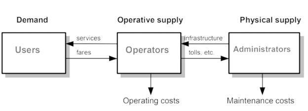
The primary components of the TRANS model of the transport system are demand, operative supply, and physical supply. Demand is the need for mobility derived from the activity model. Operative supply represents the services or amenities that can be operated and used, such as cars, trucks, railways, etc. Physical supply is related to the transportation infrastructure for the transportation of goods and people, such as roads, sidewalks, public transit, etc. The interaction between these three components centers on users’ demand for services and paying the associated costs. In turn, operators must continue operating and pay their costs. Tolls are an excellent example of such a trade-off. Similarly, administrators may charge the operators and should be responsible for paying the maintenance costs (Modelistica, 2005). Figure 8.4 shows the relationship between the model’s three primary components:

The connection between various agents in TRANUS model, that is users, operators, and administrators. — **Figure 8.4** *The Interaction Between Users, Operators, and Administrators in TRANUS.* From “TRANUS: Integrated Land Use and Transport Modeling System; General Description,” by T. Barra, 2021, *Modelistica*, p.8. In the public domain.

The rest of the procedure for the transport sub-model follows the general and conventional procedure of four-step transportation modeling. This model will be described extensively in the final chapters of this book.

TELUM

The Transportation Economic and Land Use Model (TELUM) is a model sponsored by the Federal Highway Administration (FHWA) and built on the Putman framework (Kockelman, 2008). TELUM is suitable for both short-term and long-term assessments of transportation planning projects and land-use policies, such as future employment locations and households. Rewrite for clarity. For example, it can assist in assessing the consistency implications of land use and transportation on air quality over time.

Like previous models, TELUM has three sub-models: TELUM-EMP, TELUM-RES, and LANCON. Each sub-module helps forecast the employment location (-EMP), residential location (-RES), and total land consumption (LANCON) in each zone according to its demand and supply.

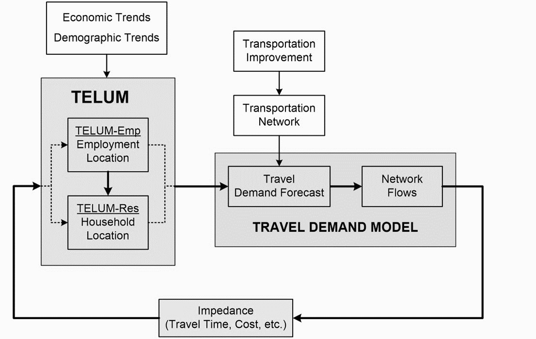
This modeling package was introduced in 2006 and is a computer-based system developed to help decision-making for small and medium-sized Metropolitan Planning Organizations (MPOs). More specifically, using this model, planners can observe the change in land-use patterns as a function of changes to the transportation infrastructure. As a result, TELUS can test the implications of various programs or policies on land use and growth patterns (Golias et al., 2014). Similar to the previous models, TELUM can also internalize the conventional four-step model (FSM), and its output can be the input for the four steps of travel demand modeling. Accordingly, Figure 8.5 shows the schematic structure of TELUM that integrates various data from employment, land use, and transportation.

TELUM model consisting of socio-demographic trends, employment and household data, and travel demand modeling. — **Figure 8.5** *Schematic Structure of TELUM.* From “TELUM: Interactive Software for Integrated Land Use and Transportation Modeling” by L. Spasovic, 2013, New Jersey Institute of Technology. p.9. In the public domain.

TELUM package consists of a total of five modules or sub-models which are introduced here:

(i) IDEU: a module for initial data entry

(ii) DOPU: the second module, which is developed for data organization and preparation

(iii) TIPU: the third module, related to transportation data and processes data about travel impedance

(iv) MCPU: the fourth module, which is utilized for calibration purposes

(v) MFCU: is the final step or module, used for model forecasting

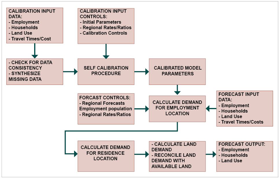
Based on the five modules, which are the essential components of the model, the modeling process can be visualized as Figure 8.6 shows:

Iterative framework of TELUM model that consists of, employment and household data, and land use. — **Figure 8.6** *TELUM Modeling Process.* From *TELUM: Interactive Software for Integrated Land Use and Transportation Modeling*, by L. Spasovic, 2013, New Jersey Institute of Technology. p.11. In the public domain.

TELUM Data requirements

The TELUM model requires ten data types to successfully run the model:

Employment data,
Household data,
Land use data,
Household-employment conversion ratio,
Number of workers per household in each income category,
Unemployment rate,
Net commuting rate,
The total number of jobs per region,
Projected zonal totals, and
Travel impedance.

Additionally, lagged year data is also necessary for the calibration task. The time interval suggested by the model developer and other resources for the model is a 5-year increment (Kockelman, 2008).

Table 8.1 summarizes all categories of data needed for TELUM and popular sources for obtaining them.

**Table 8.1** Data Requirements for TELUM. Note. Table From “*Land Use Forecasting Models for Small Areas in North Carolina*” by B. Morton, 2013, North Carolina Department of Transportation. p.7. In the public domain.
Datum	Source
Total population for lag year (by zone) +	Census or American Community Survey
Total households for lag year (by zone)	Census or American Community Survey
Households for current year (by zone and sector)	Census or American Community Survey
Group quarters population for current year (by zone)	Census or American Community Survey
Total employed residents for current year (by zone, i.e., place of residence)	Census or American Community Survey
Employment for lag year and current year (by zone, i.e., place of work, and by sector)	Census or American Community Survey
Land occupied by residences for current year (by zone)	Local government’s parcel data
Number of jobs per employee (for study area)	Local government or council of governments
Net commuting rate (for study area)	Census or American Community Survey
Unemployment rate (by sector for study area)	Employment Security Commission
Employees per household (by sector for study area)	National Household Travel Survey
Land occupied by industrial establishments for current year (by zone)	Local government’s parcel data
Land occupied by commercial establishments for current year (by zone)	Local government’s parcel data
Land devoted to transportation infrastructure for current year (by zone)	NC DOT
Vacant, developable land for current year (by zone)	Local government’s parcel data
Unusable land for current year (by zone)	Local government’s parcel data
Zone-to-zone travel times and/or costs for current year	Travel demand model
Total population (for study area)	Census or state demographer
Total employment (by sector for study area)	Woods & Poole Economics, Inc.
Unemployment rate (for study area)	Judgmental extrapolation from base year
Employees by household (by sector for study area)	Judgmental extrapolation from base year
Average income per employee (by sector for study area)	Judgmental extrapolation from base year
Jobs per employee (for study area)	Judgmental extrapolation from base year
Zone-to-zone travel times and/or costs for current year	Travel demand model

When modeling with TELUM, data preparation and cleaning is required before running the model, including:

The employment data needs to be divided into classes (minimum of four and maximum of eight) for both the base and lagged years.
Divide the zonal household data into a minimum of four household classes and a maximum of eight (preferably based on income).
Categorize the total land into usable and unusable land in each zone.
Divide the usable land into basic employment, service employment, residential land use, and vacant land.
Specify an employment-to-household conversion ratio for each of the employment and household classes. If the data is not available, an even distribution is assumed.
Determine the average number of employees living in each household group in each zone.
Specify the unemployment rate. The assumption is that unemployed households chose their residential location when employed. If not available, this rate can be assumed to be zero.
Determine the net commuting rate based on the number of work trips in and out of the region.
Determine the total number of reported jobs. If unavailable, replace this data with the total number of employees.
Predict the population and employment classes for the forecasting year.
Create zones based on the average population of each zone in the range of 3,000 to 10,000 persons.
Create the trip matrix of travel cost or time between each pair of zones.

TELUM OUTPUTS

In addition to data preparation and organization, we should also determine the calibration process for specific parameters based on local data. Rewrite for clarity. Apart from preparing and organizing the data, it is crucial to establish the calibration process for specific parameters using local data. The TELUM-EMP requires calculation of five parameters for each employment category. TELUM-RES and LANCON, require calibration of six and 19 parameters, respectively. It is also worth mentioning that the methodology for modeling the data to best fit in TELUM utilizes non-linear methods (Kockelman, 2008). After accomplishing the model calibration task and validating the accuracy of these values, the model can generate preliminary forecasts. Table 8.2 summarizes the initial results of the model as well as the application of the forecasts for planning implications.

**Table 8.2** TELUM Results and Planning Implications. Note. Table created by authors.
Output	Planning Implications
Employment Density (forecasted for each zone and employment category)	Use: estimating future payroll tax revenues, change of zoning/land use and improvements of the transportation network to promote desired development scenario.
Household Density (forecasted for each zone by household income category)	Use: estimating future property taxes, change of zoning/land use and improvements of the transportation network to promote desired location of residencies throughout the region.
Land Consumption (forecasted for each zone by household/employment category)	Use: provides an estimate of intensity of land utilization by households and employment by category, indicating how land use will change as a result of location of population and jobs for different development scenarios.
Density Gradient (measure of urban sprawl)	Use: by measuring change in household density as one moves from the CBD to suburbs can help identify trends in long-range regional plans

TELUM allows planners to test the implication of various programs and policies on urban growth, land use patterns, land consumption, transportation network performance, etc. rewrite for clarity. Modeling different scenarios and alternatives allows planners to compare the impacts of various programs.

The TELUM software package is free, intuitive, and interactive, with many user-friendly features. The results are easy to understand, and data entry is a relatively simple task with numerous tools provided within the model. Since TELUM produces disaggregated population and employment forecasts by job and household type, several measurements for accessibility for different job types and population categories are possible (Merlin et al., 2018). One of the key advantages of TELUM is readily available input data, mainly from U.S. Census data and supplementary data available from local MPOs. Also, it is possible to integrate a GIS (Geographic Information System) module, which enables the modeler to map the input data, calibration results, and final forecasts. However, TELUM is not equipped and integrated with travel demand models. This shortcoming limits synchronization between the two estimations (Merlin et al., 2018).

PECAS

Thus far, we have explored three integrated land-use and transportation models, their underlying concepts, and the necessary steps for implementation. Two different model structures are distinguishable for integrated land-use and transportation models. One type looks for a unifying principle for modeling and tries to integrate all sub-systems. The other type considers the urban area as a hierarchical system of interconnected but autonomous sub-systems. The former is called unified, and the latter is composite (Hensher, 2004). In this chapter, the first two models, MEPLAN and TRANUS, belong to the unified category, while TELUM is a composite model. This section will discuss PECAS (Production, Exchange, and Consumption Allocation System), which is another unified model. An important structural distinction between TELUM and PECAS is that the latter is much more data intensive.

PECAS is an approach for forecasting spatial economic systems and results in the simulation of land-use consumption. This aggregate and dynamic equilibrium structure simulates the flows of exchanges (i.e., goods, services, labor, and space) based on technical coefficients and market clearing, all of which are exogenous to the model (Hunt et al., 2005). Nested logit models allocate these flows using price and transport impedances. After that, simulation outputs are converted into travel demands. Then the demands are assigned to the network, following which new impedances are calculated iteratively. Finally, the prices determined for space will inform the calculation of space changes (land-use change pattern), thereby simulating developer actions and land-use development decisions (McCoy, 2009). In an iterative process, travel impedances or disutility and changes in space for year n will influence the flows of exchange in the year n+1 (Hunt et al., 2005). PECAS is a generalization of the spatial input-output modeling in MEPLAN and the TRANUS land-use transport modeling system (Hunt et al., 2005).

PECAS Sub-models

Two sub-models perform the data analysis in PECAS: the activity allocation (AA) model and the space development (SD) model. We must have a time increment of one year, and land use zones should be at most 750.

The Activity Allocation Module explores and analyzes how activities find their optimum location and interact with one another. This module assumes that the flow of commodities is a two-part trip with three points. One trip is from the production point to the exchange point, and another is from the exchange point to the consumption point, defining a three-level nested logit model. The highest level in the nested structure allocates the total activity within the study area to land use zones. The middle level distributes each activity to each zone. The last level allocates the produced goods and services and their consumption quantity to exchange locations by defining two logit models (Kockelman, 2008). This module centers on spatially disaggregated forms of an extended input-output table (aka social accounting table) as the input data. Labor (employment) is also considered a commodity produced by households and consumed by economic activities. Similarly, floor space is considered a commodity that activities consume, and its amount is fixed in each zone at any given time. Here, floor space is a static commodity for which the exchange and consumption location is the same.

Like previous models, calibration is a pivotal task in PECAS, and in the activity allocation module, the following data is needed for calibration:

The input-output matrix for the base year, along with import and export information;
The technical coefficient in the input-output matrix for the base year (such as land consumption rate);
Distribution of employment disaggregated by sector and occupation;
Labor force participation rates disaggregated by household type and occupation for the base year;
Trip length distribution for each commodity in the base year; and
The average price for each commodity, the variation of the price, and indications of where the price is higher and where it is lower (Hunt et al., 2005).

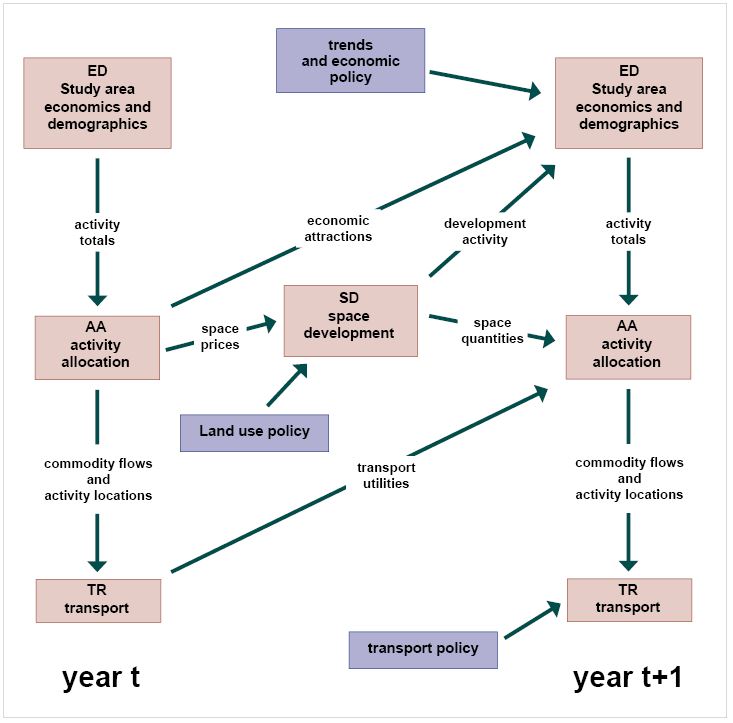
Figure 8.7 illustrates the general structure of the PECAS model and the role of its sub-models.

This photo shows the framework of PECAS between two time intervals — **Figure 8.7** *PECAS* *Model Structure.* Adapted from “Design and Implementation of PECAS: A Generalised System for Allocating Economic Production, Exchange and Consumption Quantities,” by J.D. Hunt, J.D. Abraham, in (Ed.), *Integrated Land-Use and Transportation Models* (p. 3), 2005, Emerald Publishing Group. Copyright 2016 by Emerald Group Publishing Limited.

The activity allocation module represents developers’ decisions for developing spaces for different activities from one time to another. Rewrite for clarity. It is an aggregate-based module that employs a set of logit models to model the change in quantities of space in each category for each land-use zone from one time period to the next. (McCoy, 2009). Total land or space can fall into the following categories: (1) existing floorspace and land, (2) serviced vacant land (infrastructure), or (3) unserviced vacant land. Through the model, a logit model would help calculate the quantity to allocate to each of the following discrete alternatives: (i) remaining in the same space category, (ii) becoming derelict, or (iii) transforming into other types.

Furthermore, the data needed for the calibration process in this module includes:

Transformation or change in the space allocated to each category between base and forecasting year, and
Supplementary information for each zone for the base year, such as zoning regulations, construction costs, and quantities of unserviced and serviced vacant land.

PECAS, as mentioned earlier, is a data-intensive model that provides a means for the modeler to gain insights into specific data requirements. It not only simulates future interactions between various economic sectors and categories but also addresses land-use patterns. Similar to MEPLAN and TRANUS, PECAS is a unified land-use and transportation-integrated model.

However, the biggest challenge in using PECAS is model calibration, which is an onerous task. This is because, as we saw, there are several data needs for calibration and many coefficients whose values are to be determined. The interactions between model elements that influence and are influenced by these coefficients are complex. PECAS is developed so that a comprehensive modeling framework would be utilized rather than limiting the model form so that it is consistent with available data. The synthesis of diverse data, as emphasized in PECAS requirements, is crucial because not all types of data are readily available (Hunt et al., 2005).

Conclusion

In this chapter, we reviewed four integrated land use and transportation models, all based on the feedback loop or interactions between land and activity market and transportation costs or systems. As mentioned in chapter 2, these models are based on the concepts of social physics and seek for an equilibrium state in the iterative function of the model. Furthermore, these models assume that relationships between utilities of different choices and contributing factors are linear based on past data. However, agents like households or businesses may factor in other features or feature trends in their decisions. That said, since these models employ highly disaggregate representations of urban economy by separating different jobs and business using I-O matrices for a long-term period, they proven to be accurate in forecasting when the impacts of projects should be most anticipated. For instance, using TELUM, we can estimate the space-consumption elasticities through the forecasting period and inform decision-making for implementing different scenarios. While several planning and modeling agencies have embedded these models in their land use/transportation forecasts, newer approaches such as activity- or cell-based models are being rapidly developed for accounting for heterogeneity and practicing more bottom-up planning.

Key Takeaways

In this chapter, we covered:

Four new models (MEPLAN, TRANUS, TELUM, and PECAS) for performing an integrated land-use/transportation analysis.
Detailed descriptions of each of the four models’ framework and application of their sub-models within the model.
Detailed exploration of data requirements for each model and ways to prepare and use them within the model.

Prep/quiz/assessments

Explain the relationship between the modules of MEPLAN and the interaction between them.
What are the setbacks of the MEPLAN model? Are these setbacks expandable to other models as well?
What are the concepts of demand, operative supply, and physical supply in the TRANUS model, and their relationship?
Enlist some of the data requirements for the TELUM model and summarize the required data preparation tasks for each of them
What is the difference between the Activity Allocation and Space Allocation modules in PECAS? Explain.

References

Abraham, J., & Copyright, C. (1998). A review of the MEPLAN modelling framework from a perspective of urban economics. https://citeseerx.ist.psu.edu/document?repid=rep1&type=pdf&doi=478b3f33497bf8a9a62ca3508150975df994dd93

Abraham, J. E., & Hunt, J. D. (1999). Policy analysis using the Sacramento MEPLAN land use–transportation interaction model. Transportation Research Record: Journal of the Transportation Research Board, 1685(1), 199–208. https://doi.org/10.3141/1685-25

Briassoulis, Helen. 2020. Analysis of land use change: Theoretical and modeling analysis of land use change: Theoretical and modeling approaches approaches. WVU Research Repository, 2020. https://researchrepository.wvu.edu/cgi/viewcontent.cgi?article=1000&context=rri-web-book

Domencich, Thomas A, and Daniel McFadden. 1975. “Urban travel demand-a behavioral analysis Trid.trb.org. https://trid.trb.org/view/48594

Echenique, Marcial H, Anthony DJ Flowerdew, John Douglas Hunt, Timothy R Mayo, Ian J Skidmore, and David C Simmonds. 1990. “The MEPLAN models of Bilbao, Leeds and Dortmund.” Transport Reviews 10 (4): 309–22. https://doi.org/10.1080/01441649008716764

Feudo, F. L., Morton, B., Capelle, T., & Prados, E. (2017, December 9). Modeling urban dynamics using LUTI Models: Calibration methodology for the Tranus-based model of the Grenoble Urban Region. Hong Kong, China. https://hal.science/hal-01666452

Golias, M., Mishra, S., & Psarros, I. (2016). A guidebook for best practices on integrated land use and travel demand modeling. Tennessee Department of Transportation. https://trid.trb.org/view/1398494

Hensher, David A. 2004. Handbook of transport geography and spatial systems. Elsevier.

Hunt, J. D., & Abraham, J. E. (2005). Design and implementation of PECAS: A generalized system for allocating economic production, exchange and consumption quantities. In Lee-Gosselin, M.E.H. and Doherty, S.T. (Ed.) Integrated Land-Use and Transportation Models, Emerald Group Publishing Limited, Bingley, pp. 253-273. https://doi.org/10.1108/9781786359520-011

Hunt, J. D., Kriger, D. S., & Miller, E. J. (2005). Current operational urban land-use-transport modelling frameworks: A review. Transport Reviews, 25(3). https://trid.trb.org/view/768914

Kockelman, K. (2008, August 31). Examination of land use models, emphasizing UrbanSim, TELUM, and suitability analysis. Texas. Dept. of Transportation. Research and Technology Implementation Office & University of Texas at Austin. Center for Transportation Research, Eds.. ROSA P. https://rosap.ntl.bts.gov/view/dot/16737

Li, W. (2015). Planning for land-use and transportation alternatives : towards household activity-based urban modeling for sustainable futures. Doctoral dissertation, MIT https://dspace.mit.edu/handle/1721.1/97799

Lowry, I. S. (1964). A Model of Metropolis. Rand Corp Santa Monica CA. https://www.rand.org/pubs/research_memoranda/RM4035.html

McCoy, M. (2009). California PECAS model development. California Department of Transportation. https://trid.trb.org/view/1410974

Merlin, L. A., Levine, J., & Grengs, J. (2018). Accessibility analysis for transportation projects and plans. Transport Policy, 69, 35–48. https://doi.org/10.1016/j.tranpol.2018.05.014

Modelistica. (2005). TRANUS: Integrated Land Use and Transport Modeling System. Manual to the TRANUS model and reporting programs.

Morton, Brian J. 2013. “Land use forecasting models for small areas in North Carolina.”, North Carolina Department of Transportation, Raleigh, NC.

Pozoukidou, Georgia. 2018. Modeling urban dynamics: the case of periurban development in east Thessaloniki. European Journal of Environmental Sciences 8 (1): 23–30.https://doi.org/10.14712/23361964.2018.4

Putman, S. 2005. “User manual: TELUM transportation economic land use model, Version 5.” Delaware: SH Putman Associates.

Spasovic, LN. 2013. “TELUM-Interactive Software for Integrated Land Use and Transportation Modeling. New Jersey Institute of Technology.”

Waddell, P. and Ulfarsson, G.F. (2004), “Introduction to Urban Simulation: Design and Development of Operational Models”, Hensher, D.A., Button, K.J., Haynes, K.E. and Stopher, P.R. (Ed.) Handbook of Transport Geography and Spatial Systems (, Vol. 5), Emerald Group Publishing Limited, Bingley, pp. 203-236. https://doi.org/10.1108/9781615832538-013

License

Icon for the Creative Commons Attribution-NonCommercial-ShareAlike 4.0 International License

Transportation Land Use Modeling and Policy (TLUMP) Copyright © 2024 by Qisheng Pan and Soheil Sharifi is licensed under a Creative Commons Attribution-NonCommercial-ShareAlike 4.0 International License, except where otherwise noted.