5 Using Models
Chapter Table of Contents
Models in General
Industrial Engineers, and other engineers, often want to perform experiments on real systems, but such experimentation can be difficult. If an IE wants to try a new layout for a production system, moving equipment, furniture, and offices would be difficult and time consuming. Even trying a new procedure may disrupt the production system. Therefore, the IE would create a model of the system, usually a mathematical model.
The following figure shows how models are used.
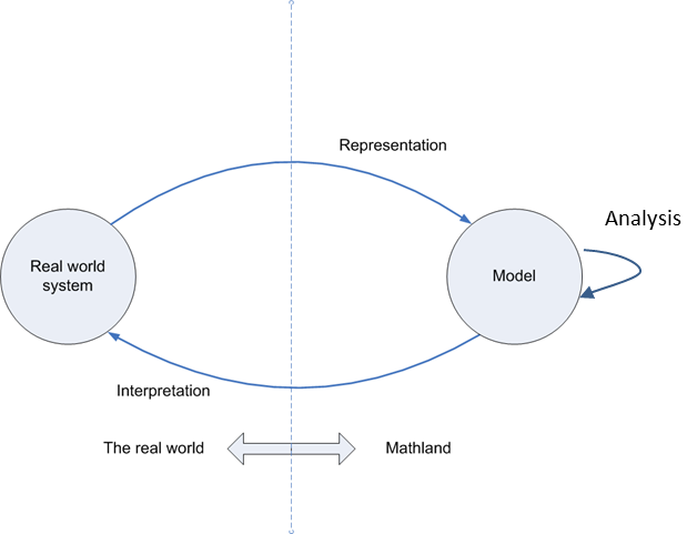
Let’s look at each piece of the diagram. The first circle is labeled “real world system.” Drawing a line around some system involves deciding which parts are in your system and which are in the environment. For example, to study the arrival and service of customers at a bank, you would probably include the tellers, the drive up window, and the ATM, but not include the roads and traffic system that people use to get to the bank.
The second circle is labeled “model.” Some types of engineers use physical models. For example, a civil engineer might place a scale model of a building on a shaking table to predict how the building will respond to an earthquake. IEs tend to use mathematical models, expressed in equations or sometimes in computer code. For example, an IE might use the mathematics of queuing theory to create a model of the bank.
The top arrow labeled “representation” reminds us that the model represents the real world system but only the relevant parts of the system. Our model of the bank must include information on the time between customer arrivals and the time to serve each customer (both of these times vary from customer to customer), but the model doesn’t have to include descriptions of what color clothing customers wear. Depending on the purpose of our model it might include information on customer’s disabilities so we can predict how many teller windows must be accessible to people in wheelchairs. The M/M/1 queuing model describes the time between arrivals as an exponential random variable with average 1 customer/λ (say 6 minutes) and the time of service as an exponential random variable with average 1 customer/μ (say 4 minutes).
A model is never exactly correct; you should always remember the phrase “it’s only a model.” For example, the M/M/1 queuing model assumes that customers arrive at the average rate of 1 customer every 6 minutes, or 10 customers per hour. Actually, the arrival rate probably varies over the day.
An IE creates a model in order to extract information; the loop from the model to itself is labeled “analysis.” IEs use some models quite frequently and IEs can use mathematical results that others have proven. For example, for the M/M/1 queuing model can be used to compute the average number of people in the queue.
The line labeled “interpretation” is where the IE interprets the mathematical results of the model back to the real world system. Now the IE must again remember “it’s only a model” so the predictions may not be perfect. Since the M/M/1 queuing model assumes a constant average arrival rate, the results using λ = 10 customers per hour can only be applied to the period of the day with that arrival rate. A separate model might be needed for the lunch hour, which is probably busier.
IEs are responsible for efficiency, including the efficient use of time and resources. You already know from calculus class how to find the maximum or minimum of a function and calculus is one tool that IEs use. However, IEs often need to maximize or minimize a linear function, which sounds easy, but finding the solution isn’t easy when there are many variables and also some constraints. The following is an example of such a problem.
Dairy cattle have various nutrient requirements, such as protein, calcium, and potassium, that can be met by different types of feed, such as alfalfa, hominy, and corn cobs. The dairy farmer wants to mix a feed for the dairy cows that will meet the nutrient requirements at the minimum cost. Below is a very simplified version of the Diet Problem as applied to feeding dairy cattle. The following table gives the nutrient content (protein and potassium) of certain feeds (alfalfa, hominy, and corn cobs), as well as the nutrient requirement for protein and potassium (as a percent of the feed) and the cost of alfalfa, hominy, and corn cobs (in $/ton).
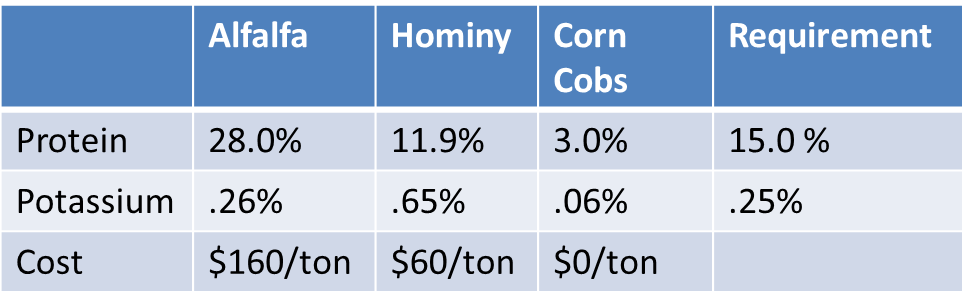
For example, alfalfa is 28% protein, 0.26% potassium, and costs $160 per ton. Alfalfa is a good source of protein and a medium source of potassium, but it is expensive. Hominy is a medium source of protein and a good source of potassium, and it is cheaper than alfalfa. Corn cobs are not a good source of either protein or potassium, but since they are otherwise a waste product, they are free. With some thought, you can see that the optimal mix will probably need alfalfa to meet the protein requirement, hominy to meet the potassium requirement, and corn cobs to keep the cost down.
We want to determine how to mix the feed, that is, what fraction should be alfalfa (A), hominy (H), and corn cobs (C). We will use linear programming to solve this problem, by expressing the situation as minimizing a linear objective function (cost) subject to linear constraints (protein and potassium). Because the ingredient’s units are representing percentages of the whole, we also know that A+H+C=1.
Here is the linear programming formulation:
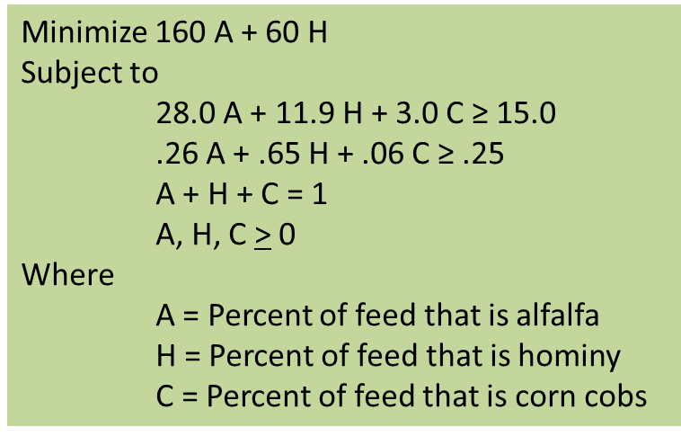
This model is an example of a linear programming model. We can solve it mathematically. There are also computer programs that can help us to solve this type of problem. Excel is one such program although there are better tools for solving LP models.
This problem is an example of how industrial engineers use mathematics to promote efficiency. In this case, we helped the farmer use his or her resources efficiently to keep the cattle healthy while minimizing the cost of feed. This model is an example of an LP model, or, more broadly, an example of a deterministic optimization model. “Deterministic” means the model has no probabilities and “optimization” means we found the optimal, or best, solution.
An LP model is just one type of deterministic optimization model. Actually, in this example we assumed that we can buy any real amount of ingredients. If it were necessary to buy only in integer quantities a LP would not be an appropriate model. An model where the decision variables must be integers is called an integer programming model (IP).
Industrial engineers must be able to recognize situations where a deterministic model can be applied, create an appropriate model, and solve the model using an appropriate tool. The following list describes situations where a deterministic optimization model might be useful.
- Product mix – determine how much of each type of product to make subject to constraints on available resources.
- Production scheduling – determine how much of each type of product to make in different time periods in order to meet specified production amounts by certain times.
- Blending – determine the best blend of inputs to use to minimize the cost of producing a mixture. Our feed example was a blending model.
- Cutting stock – determine the best way to cut resource material to maximize profit. For example, a log can be cut into lumber of various dimensions which can be sold for different amounts.
- Staffing – determine the best way to assign people to jobs to maximize their preference or to maximize the productivity, based on their abilities at different jobs.
- Transportation – determine the best way to route resources through a transportation network to minimize the cost, while delivering the appropriate amount of resources to each location.
- Assignment – determine the best way to assign resources to tasks.
- Traveling salesman problem – determine the best route among a number of points that visits each point at least once.
