4 Basic Data Analysis
4.1. Overview
This chapter covers the steps for preparing secondary data for statistical analysis and how to run common statistical tests. The reader will be introduced to some basic data analysis procedures using SAS 9.4. It is important to follow the steps for preparing secondary data for statistical analysis to ensure accuracy, particularly when using numerous years or combining multiple data files within each year. The examples in this chapter will use data from the 2018 National Health Interview Survey (NHIS) Sample Adult file. The examples will demonstrate ways to answer the following two research questions among adults ages 18 and older in the United States (US):
- Research Question 4.1: What are the associations between region (geographic location where participant lives) and health information technology (HIT) usage?
- Research Question 4.2: What is the association between sex and HIT usage?
The NHIS includes five questions to measure individuals’ use of different aspects of HIT usage during the past 12 months, including whether or not adults use computers to fill prescriptions, schedule appointments, communicate with others through chat groups, look up health information online, and communicate with health care providers by e-mail.1 The primary author of this textbook (Kindratt) and colleagues have used NHIS data to explore how HIT usage influences vaccination and cancer screening uptake.2,3 The examples in this chapter will focus on differences by sociodemographic factors, such as place of residence and sex. SAS 9.4 procedures will be used to demonstrate how to meet the following research objectives using common statistical tests.
- Objective 4.1: To determine the association between region and looking up health information on the internet
- Objective 4.2: To determine the association between region and filling prescriptions on the internet
- Objective 4.3: To determine the association between region and scheduling appointments on the internet
- Objective 4.4: To determine the association between region and communicating with health care provider by e-mail
- Objective 4.5: To determine the association between sex and the number of HIT uses (scale from 0 to 4)
- Objective 4.6: To determine the associations between sex and each HIT use (looking up health information online, filling prescriptions, scheduling appointments, and communicating with a health care provider by e-mail) before and after controlling for other contributing factors
It is important to note that the examples provided in this chapter are not weighted and do not include procedures for adjusting the results based on the complex survey design. Therefore, estimates you obtain as the results are not representative of the true findings. The complex sample design features that should be used when analyzing national health data will be described in Chapter 5.
4.2 Four-Step Process for Secondary Data Analysis
When preparing secondary data for statistical analysis, it is important to follow these steps to ensure accuracy and completeness of your data. This 4-step process was developed based on recommendations from Elliot and colleagues for preparing and managing primary data in Microsoft Excel and Database Creation and Coding sessions by Kindratt for training medical and physician assistant students.4-6 The four steps include: 1) data selection; 2) data collection; 3) data verification; and 4) data storage.
4.2.1 Data Selection
The first step is data selection, which is the process of determining the appropriate data type and source, as well as suitable instruments to collect data. Once a research question has been solidified, the next step in secondary data analysis is to determine the appropriate data source. For this example, the research question focuses on differences in where adults live in the US and their HIT use. Since the NHIS is one of the largest national surveys that collects this information and provides publicly available data, it is a good selection to answer this research question.
4.2.2 Data Collection
The second step is data collection, which is the process of gathering and measuring information on variables of interest in an established and systematic fashion that enables one to answer stated research questions and test hypotheses. For secondary data analysis, data collection procedures include downloading the necessary data file and supporting documentation from websites and collecting data from only the variables needed to answer the research question and objectives. The 2018 NHIS Sample Adult file and Sample SAS statements can be downloaded from the NHIS data release website.
To collect the appropriate variables for this analysis, complete the following:
- Go to your “C:\” drive and create a folder named “NHIS”
- In the “NHIS” folder, create a folder named “18”
- Download the 2018 Sample Adult ASCII data file (.dat) from the 2018 NHIS data release website
- Unzip the file and save it in the folder “C:\NHIS\18”
- Download “File 4.1 Sample SAS Program to Create NHIS 2018 Sample Adult File” from the Open ICPSR data repository
- Open the file and select “Run” from the top menu bar
Your analytic dataset should include the following 9 variables:
- SRVY_YR
- FPX
- AGE_P
- SEX
- REGION
- HIT1A
- HIT2A
- HIT3A
- HIT4A
To verify the variables in the analytic dataset, run the PROC CONTENTS statement in Box 4.1.
Box 4.1. SAS procedure (PROC CONTENTS) for verifying the variables included in the 2018 NHIS Sample Adult example analytic dataset

If you are unable to create the permanent analytic dataset using the preceding steps, click on “File 4.2 Permanent SAS Analytic Database” to download and save the database in the folder “C:\NHIS\18.”
4.2.3 Data Verification
The third step is data verification, which involves verifying that the results from the analytic dataset you created match those provided by the original dataset. Most national health surveys, including the NHIS, provide at least unweighted frequency counts for you to match your findings with those published on the website. Other national health surveys, such as the Medical Expenditure Panel Survey, provide more detailed information like weighted frequencies and percentages. The frequency verification should be completed prior to making any changes to the variables you collected for your analysis. Your results will not match if you verify the frequencies after applying any limitations to the data. For example, if your sample only includes adults ages 45 and older, I recommend that you verify the results for adults ages 18 and older prior to removing individuals ages 18-44 years to ensure the accuracy of the analytic dataset.
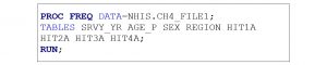
In this example, you can view the unweighted frequencies for variables you collected by going to the 2018 NHIS data release website and clicking on “Variable frequencies” in the “Sample Adult File” section. You should be able to search for each variable by clicking “Ctrl” and “F” and typing the name of the variable into the search box. You will need to run frequencies for each variable of interest in SAS to verify results. PROC FREQ is the procedure for displaying frequencies in SAS. You can enter the SAS syntax from Box 4.2 to determine the frequencies for all variables in the analytic dataset. Variable FPX is excluded because it represents the ID number of the participant.
Box 4.2. SAS procedure (PROC FREQ) for verifying frequencies in the 2018 NHIS Sample Adult example analytic dataset
The unweighted frequencies for the variables collected in this example are presented in Table 4.1. The variable for age (AGE_P) is excluded from the table due to multiple response options (age 18-85 years and older).
Table 4.1. Frequencies for data collected in the 2018 NHIS Sample Adult example analytic dataset
| Variable Description (VARIABLE NAME) | Frequency |
|---|---|
| Survey Year (SRVY_YR) | |
| 2018 |
25,417 |
| Sex (SEX) | |
| 1=Male |
11,550 |
| 2=Female | 13,867 |
| Region (REGION) | |
| 1=Northeast |
4,143 |
| 2=Midwest | 5,949 |
| 3=South | 9,312 |
| 4=West | 6,013 |
| Looked up health information on internet, past 12 months (HIT1A) | |
| 1=Yes |
13,677 |
| 2=No | 11,431 |
| 7=Refused | 11 |
| 8=Not ascertained | 273 |
| 9=Don’t know | 25 |
| Filled a prescription on internet, past 12 months (HIT2A) | |
| 1=Yes |
2,892 |
| 2=No | 22,240 |
| 7=Refused | 6 |
| 8=Not ascertained | 274 |
| 9=Don’t know | 5 |
Table 4.1 (continued). Frequencies for data collected in the 2018 NHIS Sample Adult example analytic dataset
| Variable Description (VARIABLE NAME) | Frequency |
|---|---|
| Scheduled medical appointment on internet, past 12 months (HIT3A) | |
| 1=Yes | 3,962 |
| 2=No | 21,163 |
| 7=Refused | 7 |
| 8=Not ascertained | 274 |
| 9=Don’t know | 11 |
| Communicated with health care provider by email, past 12 months (HIT4A) | |
| 1=Yes |
4,176 |
| 2=No | 20,948 |
| 7=Refused | 7 |
| 8=Not ascertained | 274 |
| 9=Don’t know | 12 |
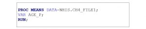
For continuous or discrete variables with multiple responses (variable: AGE_P), summary statistics can be used to verify the measure of central tendency (mean), measure of dispersion (spread), range, and total number of responses. PROC MEANS is the procedure used for displaying the mean and standard deviation. You can enter the SAS syntax from Box 4.3 to determine the mean and standard deviation for AGE_P in the example analytic dataset.
Box 4.3. SAS procedure (PROC MEANS) for verifying continuous/discrete variable distributions in the 2018 NHIS Sample Adult example analytic dataset
4.2.4 Data Storage
The fourth step is data storage. When using secondary data from publicly available sources, it is important to save the original datasets that you downloaded from the website. This helps ensure that you always have your data in case the website address changes or there is a change in policy that prohibits you from accessing the data at no cost. For restricted data, you must follow the rules for data storage set forth by the agency that owns the restricted data. You may not be able to keep the data over a certain period of time and you may be asked to destroy any outputs with results after the publication of your research.
Each time you make changes to your analytic dataset in SAS, you can save the data using the following two ways:
- “work” file
- “permanent” file
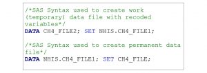
The work file is temporary and will only be saved for the current analysis. A limitation of creating a work file is that you will have to re-run the code again each time you use the data if you made any changes to the file (i.e. create recoded variables). However, some benefits to creating a work file are that it will not take up as much space on your computer and the procedures often run faster. Another benefit to saving a permanent data file is that the cleaned, recoded and organized analytic dataset is saved and available for running analyses again after your study is completed. Box 4.4 provides SAS coding for creating a new work file from a permanent data file and a permanent data file from a work file. The permanent file includes a libname in front of the temporary file name (e.g. NHIS.ch4_file1 (permanent) vs. ch4_file (work)).
Box 4.4. SAS programming statements to create work and permanent analytic datasets
4.3 Common Statistical Tests
Prior to choosing the type of statistical test you must know the type of data collected and the variables you will use to answer your research questions and fulfil your objectives. You must know whether the data are continuous or categorical and specify the independent, dependent, and other contributing variables that will be included in the analysis.
4.3.1 Types of Data
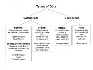
Secondary data sources can include continuous and categorical variables. Continuous variables are numeric responses and can be ratio (with a meaningful zero, such as height) or interval (without a meaningful zero, such as temperature). Continuous responses may be subjective (e.g. self-reported), objective (e.g. clinically measured) or both measurements. Categorical variables include nominal and ordinal responses. Nominal responses include categories that do not have a more or less than relationship. A nominal variable for the example used in this chapter is “REGION.” The US region where an individual resides includes the following values: 1=Northeast; 2=Midwest; 3=South; or 4=West. An individual who lives in the West region is not any better than someone who lives in the South region. Binary, also referred to as dichotomous, responses represent variables with only two options. A binary variable for the example used in this chapter is “SEX.” The sex of each individual is represented as 1=male and 2=female. There is no more or less than relationship between males and females. Each measure of HIT use can also be represented as a binary variable once the responses for 7=Refused, 8=Not Ascertained, and 9=Don’t Know are removed/made missing. Each recoded variable for HIT use with 1=Yes and 0=No responses will then be binary/dichotomous. Ordinal or ranked variables represent data that have a more or less than relationship. Variables must include at least three categories. An ordinal variable for the example in this chapter can be created by adding up all of the HIT uses of participants to determine the total number of HIT uses (0=Does not use any health information technology to 4=Use the internet to look up information, fill prescriptions, schedule appointments, and communicate with a health care provider by email). Other common examples of ordinal variables are Likert scales of agreement (1=strongly disagree to 5=strongly agree) and smoking status (0=never, 1=former, 2=current). An overview of the types of data used for research using national health surveys is provided in Figure 4.1.
Figure 4.1: Flowchart of types of data
The type of variable that you need to answer your research question may be different than what is available using the publicly available data files. It is common to recode variables to limit the responses based on how you want the data to be used for answering your research questions. IF/THEN programming statements can be used for recoding prior to statistical analysis. SAS syntax used to create new binary variables and an ordinal HIT usage variable is provided in Box 4.5.
Box 4.5. SAS programming statements (IF/THEN) for recoding secondary data
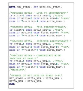
In Box 4.5, each HIT use variable has been recoded to a binary variable with “_NEW” added to the end of the original variable name (e.g. HIT4A_NEW for yes/no responses to communicating with a health care provider by e-mail in the past 12 months). A new ordinal variable named HIT_SCALE was created to represent the total number of HIT uses.
4.3.2 Types of Variables
Once the type of data is determined, the independent, dependent and other contributing variables need to be identified. The independent variable in a statistical model is the variable used determine the influence or impact on the outcome.7 The independent variable is also known as the “predictor” or “exposure” variable. In the 2018 NHIS Sample Adult example, the independent variable for research question 4.1 is region and the independent variable for research question 4.2 is sex. The dependent variable in a statistical model is the variable used as the outcome, for which differences or variations in the dependent variable are being studied.7 The dependent variable is also known as the “outcome” variable. In the 2018 NHIS Sample Adult example, the dependent variables are each individual HIT usage (looking up health information on the internet, filling prescriptions, scheduling appointments, and communicating with a health care provider by e-mail) and the HIT usage scale (0-4). Other contributing factors, such as confounders and covariates, must also be determined. Confounders are defined as any variables that are causally associated with the dependent variable, not causally or causally associated with the independent variable, but are not intermediate variables in the casual pathway between the independent and dependent variables.8 Covariates are defined as variables that are potentially related to the dependent variable.9 This term is often used to represent any contributing or explanatory factor that may bias the results. Covariates can be adjusted for during statistical analysis to reduce bias. In the 2018 NHIS Sample Adult example, a covariate is age. Other covariates often controlled for in statistical analysis include risk factors, social determinants of health, and health behaviors. Covariates may differ based on the independent and dependent variables of interest in your study.
4.3.3 SAS Procedures for Common Statistical Tests
Common statistical tests used for categorical data analysis with national health surveys include chi square, Wilcoxon rank sum (also known as Mann Whitney U) tests, and logistic regression tests.
4.3.3.a Chi Square
The Pearson chi square test is used to compare categorical independent variables and categorical dependent variables that are binary/dichotomous or nominal.7 Results pertaining to the first four research objectives mentioned in section 4.1 can be calculated by using chi square tests. As a reminder, the first four research objectives are:
- Objective 4.1: To determine the association between region (independent variable) and looking up health information on the internet (dependent variable)
- Objective 4.2: To determine the association between region (independent variable) and filling prescriptions on the internet (dependent variable)
- Objective 4.3: To determine the association between region (independent variable) and scheduling appointments on the internet (dependent variable)
- Objective 4.4: To determine the association between region (independent variable) and communicating with a health care provider by e-mail (dependent variable)
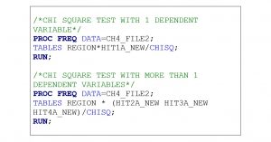
The independent (predictor or exposure) and dependent (outcome) variables are identified in each objective. PROC FREQ is the procedure used to display the crosstabulation of variables and calculation of the chi square test result. To calculate the chi square test result, you must list a “*” between the independent and dependent variable and add “/CHISQ” at the end of the statement that begins with “tables.” You can calculate the chi square test for each dependent variable separately or you can run then together.
You can enter the SAS syntax from Box 4.6 to determine the chi square test results.
Box 4.6. SAS procedure (PROC FREQ with /CHISQ) for running chi square test using the 2018 NHIS Sample Adult example analytic dataset
 4.3.3.b Wilcoxon Rank Sum/Mann-Whitney U Test
The Wilcoxon Rank Sum (also known as the Mann-Whitney U) test is used to compare differences in the medians of ordinal dependent variables among binary/dichotomous independent variables.7 The median is the center of observations when listed in rank order. The independent variable must only have two categories. For two or more categories, the Kruskal-Wallis (H) test should be used instead.7 In SAS 9.4, the coding statements for both tests are the same. The Wilcoxon Rank Sum test can be used to obtain results for research objective 4.5 in the 2018 NHIS Sample Adult example. As a reminder:
- Objective 4.5: To determine association between sex (independent variable) and the number of HIT usages (dependent variable)
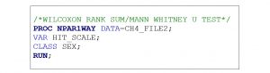
The independent (predictor or exposure) and dependent (outcome) variables are identified in the objective. PROC NPAR1WAY is the procedure used to calculate the Wilcoxon Rank Sum test result. The SAS procedure for PROC NPAR1WAY is similar to PROC MEANS. Instead of “tables” in the second line, you will use the statement “VAR” before the dependent variable (HIT_SCALE). The independent variable (SEX) is listed next to a “CLASS” statement on the next line. You can enter the SAS syntax from Box 4.7 to determine the Wilcoxon Rank Sum test result.
Box 4.7. SAS procedure (PROC NPAR1WAY) for the Wilcoxon Rank Sum test in the 2018 NHIS Sample Adult example analytic dataset
4.3.3.c Logistic Regression
Regression modeling is used to explore relations between independent (predictor) variables and dependent (outcome) variables before and after adjusting for other contributing factors that may bias the results. Logistic regression models are used when the dependent (outcome) variable is binary/dichotomous.7 Regression models that do not adjust for other contributing factors are called “crude” or “unadjusted” models. Regression models that do adjust for other contributing factors are called “multivariable” or “adjusted” models. Crude and multivariable logistic regression models can be used to obtain results for research objective 4.6 in the 2018 NHIS Sample Adult example. As a reminder:
- Objective 4.6: To determine the associations between sex (independent variable) and each HIT usage — looking up health information online, filling prescriptions, scheduling appointments, and communicating with a health care provider by e-mail — (dependent variables) before and after controlling for other contributing factors
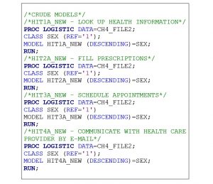
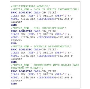
The independent (predictor or exposure) and dependent (outcome) variables are identified in the objective. The contributing factors that will be controlled for to reduce bias are region and age. PROC LOGISTIC is the procedure used to calculate the results. Enter the SAS syntax from Box 4.8 and Box 4.9 to determine the crude and multivariable results, respectively. The CLASS statement identifies the reference or comparison group for the categorical independent variable and other covariates. For the variable SEX, comparisons are made between females and males. In the analytic dataset, males are represented by “1” and females are represented by “2.” Therefore, the reference category is “1” so that our results will represent the odds of females using HIT in comparison to males. The MODEL statement is set up as “dependent variable = independent variable (+ covariates for multivariable analysis).” The DESCENDING statement after the dependent variable identifies the higher value as the outcome of interest. For each HIT use, “1=yes” should be the outcome that is modeled. Therefore, the results will indicate the odds of using HIT instead of the odds of not using HIT.
Box 4.8. SAS procedure (PROC LOGISTIC) for crude logistic regression results in the 2018 NHIS Sample Adult example
Box 4.9. SAS Procedure (PROC LOGISTIC) for multivariable logistic regression results in the 2018 NHIS Sample Adult example
4.4. Summary
This chapter provided an overview of the steps for preparing secondary data for statistical analysis and how to run common statistical tests in SAS 9.4 using primarily categorical data. The examples used in this chapter are from the 2018 NHIS Sample Adult public-use data files. The examples in this chapter focused on determining associations between demographic factors (region, sex) and HIT usage (looking up health information online, filling prescriptions, scheduling appointments, and communicating with health care providers by e-mail) among US adults. SAS 9.4 analysis procedures were demonstrated for running descriptive statistics, recoding variables, and conducting comparative statistical analyses with chi square tests, Wilcoxon Rank Sum tests, and logistic regression models. As previously mentioned, the examples provided in this chapter are not weighted and do not include procedures for adjusting the results based on the complex survey design. The use of complex sample design features for national health data will be described in Chapter 5.
4.5 References
- National Center for Health Statistics. National Health Interview Survey, 2011-2015. Public-use data file and documentation. Published August 5, 2020. Accessed August 10, 2020. https://www.cdc.gov/nchs/nhis/data-questionnaires-documentation.htm
- Kindratt T, Callender L, Cobbaert M, Wondrack J, Bandiera F, Salvo D. Health information technology use and influenza vaccine uptake among US adults. Int J Med Inform. 2019;129:37-42. doi:10.1016/j.ijmedinf.2019.05.025
- Kindratt TB, Allicock M, Atem F, Dallo FJ, Balasubramanian BA. Email Patient-Provider Communication and Cancer Screenings Among US Adults: Cross-sectional Study. JMIR Cancer. 2021;7(3):e23790. doi:10.2196/23790
- Elliott AC, Hynan LS, Reisch JS, Smith JP. Preparing data for analysis using Microsoft Excel. J Investig Med. 2006;54(6):334-341. doi:10.2310/6650.2006.05038
- Kindratt TB. Research Extension Experience in Directed Studies: Solidifying Evidence-Based Medicine Competencies Through Research Participation. J Physician Assist Educ. 2020;31(1):36-41. doi:10.1097/JPA.0000000000000291
- Dehaven MJ, Gimpel NE, Dallo FJ, Billmeier TM. Reaching the underserved through community-based participatory research and service learning: description and evaluation of a unique medical student training program. J Public Health Manag Pract. 2011;17(4):363-368. doi:10.1097/PHH.0b013e3182214707
- Jacobsen KH. Introduction to Health Research Methods: A Practical Guide. 2nd ed. Jones & Bartlett Learning; 2017.
- Szklo M, Nieto FJ. Epidemiology: Beyond the Basics. 3rd ed. Jones & Bartlett Learning; 2014.
- Field A. Discovering Statistics Using IBM SPSS Statistics. 4th ed. SAGE; 2013.
