5 Complex Survey Design Features
5.1 Overview
In Chapter 4, you learned the steps for preparing secondary data for statistical analysis and how to run common statistical tests using examples from the 2018 National Health Interview Survey (NHIS) Sample Adult public-use data. SAS 9.4 programming statements were provided to run summary statistics (frequencies, means and standard deviations), chi square tests, Wilcoxon Rank Sum/Mann Whitney U tests, and crude and multivariable logistic regression models. In this chapter, you will learn how to run statistical tests using special procedures designed to account for the complex sample designs used for national health surveys. In order to produce representative estimates using national health surveys, variables for the cluster, stratum, and weighting variables must be included using SAS SURVEY procedures. The examples in this chapter will use 2018 NHIS Sample Adult data to answer the following research questions.
- Research Question 5.1: What are associations between region and health information technology (HIT) usage among adults ages 18 and older in the United States (US)?
- Research Question 5.2: What are associations between sex and HIT usage among adults ages 18 and older in the US?
The research objectives are:
- Objective 5.1: To determine the association between region and looking up health information on the internet
- Objective 5.2: To determine the association between region and filling prescriptions on the internet
- Objective 5.3: To determine the association between region and scheduling appointments on the internet
- Objective 5.4: To determine the association between region and communicating with health care provider by e-mail
- Objective 5.5: To determine the associations between sex and each HIT usage (looking up health information online, filling prescriptions, scheduling appointments, and communicating with a health care provider by e-mail) before and after controlling for other contributing factors
SAS 9.4 SURVEY procedures will be used to demonstrate how to meet the research objectives. It is important to note that Objective 4.5 from Chapter 4 has been removed from this chapter because there are no corresponding survey procedures for the Wilcoxon Rank Sum/Mann Whitney U test at the time of this writing.
5.2 Complex Survey Design Features
The secondary analysis of national health surveys involves using advanced survey-based statistical procedures to account for the sophisticated sampling designs. Stratification, clustering, and weighting techniques must be used with Taylor Series Linearization methods, which are outlined in the data analytic recommendations for each survey. Table 5.1 provides some examples of the complex design variables for the national health surveys included in this textbook.
Table 5.1. Selected clustering, stratification, and weighting variables used for analyzing complex national health surveys
| Survey | Stratification | Clustering | Weighting |
|---|---|---|---|
| National Health Interview Survey (NHIS) | PSTRAT | PPSU | WTFA_SA |
| Medical Expenditure Panel Survey (MEPS) | VARSTR | VARPSU | PERWTF18F |
| Health Information National Trends Survey (HINTS) | VAR_STRATUM | VAR_CLUSTER | TG_all_FINWT0 |
| Behavior Risk Factor Surveillance Survey (BRFSS) | _STSTR | _PSU | _LLCP_WGT |
| National Health and Nutrition Examination Survey (NHANES) | SDMVSTRA | SDMVPSU | WTINT2YR |
5.2.1 Stratification
National health surveys use stratification methods to draw a sample from the larger sampling frame of the population. The large sampling frame is divided into mutually exclusive strata and the sample is then selected from each stratum.1 Lewis (2017) states the following three reasons for using stratification in complex national health surveys: 1) to improve representation of smaller subgroups in the population; 2) to allow for multiple modes of data collection; and 3) to improve precision of statistical estimates.1 First, stratification allows for oversampling of subgroups by race/ethnicity and among states with smaller populations. For example, the NHIS oversampled underrepresented minority populations (non-Hispanic Black, Hispanic, and non-Hispanic Asian) from 2006-2015.2 In 2016, the NHIS sample design was modified to collect larger samples in smaller states. Sample sizes were increased in the 10 least populous states and Washington D.C.2 Second, stratification allows for the use of random-digit-dialing, in-person, direct mailing, and online data collection methods to be conducted in a systematic manner. The Health Information National Trends Survey (HINTS) has used several data collection methods, including random digit dialing, direct mailing, and the recently adopted web-based data collection procedures.3 Finally, the results will be more precise with homogeneous strata collected in relation to the outcome variable.1
5.2.2 Clustering
National health surveys use clustering methods to gain large samples while reducing data collection costs. Clusters are identified in national health survey documentation as primary, secondary, and tertiary sampling units.1 Clustering allows for national health surveys to collect data on multiple individuals from each household, multiple patients attending one clinic, or multiple students from one school.1 At the state level, primary sampling unit clusters are created to select samples from large metropolitan statistical areas and counties. Within each cluster, census housing blocks are selected as secondary sampling units. Within each census block, households are selected as tertiary sampling units. For the NHIS, self-reported interview data are collected from all individuals in each household then a designated sample adult and sample child are selected from households to answer additional questions on health conditions and behaviors.4 Complex national health survey analysis procedures usually require using clustering to account for the primary sampling units.
5.2.3 Weighting
Sample weights are used to account for the underrepresentation or overrepresentation of each individual in the sample. When combining multiple years of national health surveys, the weight needs to be divided by the total years combined. Specific details and formulas on how sampling weights are calculated are provided in the analytic documentation for each complex national health survey.5
5.3 SAS Survey Procedures
To complete the following SAS SURVEY examples, data from the 2018 NHIS Sample Adult file and Sample SAS statements can be downloaded from the NHIS data release website.
Complete the following:
- Go to your “C:\” drive and create a folder named “NHIS”
- In the “NHIS” folder, create a folder named “18”
- Download the 2018 Sample Adult ASCII data file (.dat) from the 2018 NHIS data release website
- Unzip the file and save it in the folder “C:\NHIS\18”
- Download “File 5.1 Sample SAS Program to Create NHIS 2018 Sample Adult File” from the Open ICPSR data repository
- Open the file and select “Run” from the top menu bar
Your analytic dataset should include the following 12 variables:
- SRVY_YR
- FPX
- AGE_P
- SEX
- REGION
- HIT1A
- HIT2A
- HIT3A
- HIT4A
- PPSU
- PSTRATUM
- WTFA_SA
The analytic dataset should include 3 more variables (PPSU, PSTRATUM, WTFA_SA) than those collected in Chapter 4. To determine the variables in the analytic dataset, run a PROC CONTENTS statement. An example of a PROC CONTENTS statement is provided in Box 4.1 in Chapter 4. If you are unable to create the permanent analytic dataset using the preceding steps, you can go to the Open ICPSR data repository, download “File 5.3 Permanent SAS Analytic Database,” and save the database in the folder “C:\NHIS\18.”
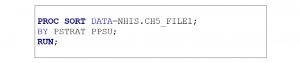
Prior to conducting survey procedures, complex survey data must be sorted by stratum and primary sampling unit variables. You can enter the SAS syntax from Box 5.1 to sort the data.
Box 5.1. SAS procedure for sorting analytic dataset by stratum and primary sampling unit
5.3.1 Survey Procedures for Frequencies and Percentages
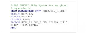
PROC SURVEYFREQ is the procedure for displaying weighted frequencies and percentages in SAS for complex surveys. Primary sampling unit, stratum, and weighting variables must be included in the programming statements. Enter the SAS syntax from Box 5.2 to determine the weighted frequencies for all variables in the analytic dataset. Variable FPX is excluded because it represents the ID number of the participant.
Box 5.2. SAS SURVEY procedure (PROC SURVEYFREQ) for determining frequencies in the 2018 NHIS Sample Adult analytic dataset
The weighted frequencies for the variables collected in this example are presented in Table 5.2. Although the NHIS does not publish the weighted frequencies in the dataset documentation on their website, other surveys, such as the Medical Expenditure Panel Survey (MEPS) and HINTS include the weighted results for data analysts to verify their outputs are correct prior to conducting additional analytic procedures.
Table 5.2. Weighted frequencies for data collected in the 2018 NHIS Sample Adult Example analytic dataset
| Variable Description (VARIABLE NAME) | Weighted Frequency |
|---|---|
| Survey Year (SRVY_YR) | |
| 2018 | 249,455,533 |
| Sex (SEX) | |
| 1=Male | 120,441,598 |
| 2=Female | 129,013,935 |
| Region (REGION) | |
| 1=Northeast | 43,261,774 |
| 2=Midwest | 54,817,888 |
| 3=South | 92,043,276 |
| 4=West | 59,332,595 |
| Looked up health information on internet, past 12 months (HIT1A) | |
| 1=Yes | 136,281,936 |
| 2=No | 110,137,528 |
| 7=Refused | 87,014 |
| 8=Not ascertained | 2,655,609 |
| 9=Don’t know | 293,446 |
| Filled a prescription on internet, past 12 months (HIT2A) | |
| 1=Yes | 28,308,262 |
| 2=No | 218,302,863 |
| 7=Refused | 59,192 |
| 8=Not ascertained | 2,666,760 |
| 9=Don’t know | 118,456 |
Table 5.2 (continued). Weighted frequencies for data collected in the 2018 NHIS Sample Adult Example analytic dataset
| Variable Description (VARIABLE NAME) | Weighted Frequency |
|---|---|
| Scheduled medical appointment on internet, past 12 months (HIT3A) | |
| 1=Yes | 41,617,782 |
| 2=No | 204,932,293 |
| 7=Refused | 67,681 |
| 8=Not ascertained | 2,666,760 |
| 9=Don’t know | 171,017 |
| Communicated with health care provider by email, past 12 months (HIT4A) | |
| 1=Yes | 41,094,984 |
| 2=No | 205,459,751 |
| 7=Refused | 67,681 |
| 8=Not ascertained | 2,666,760 |
| 9=Don’t know | 166,357 |
The variable for age (AGE_P) is excluded from the table due to multiple response options (age 18-85 years and older).
5.3.2 Survey Procedures for Means
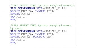
For continuous or discrete variables with multiple responses (variable: AGE_P), summary statistics can be used to verify the measure of central tendency (mean) and total responses. PROC SURVEYMEANS is the procedure used for displaying the mean and can be separated by subgroups such as region and sex. Enter the SAS syntax from Box 5.3 to determine the means for AGE_P collectively and separated by sex in the analytic dataset.
Box 5.3. SAS SURVEY procedure (PROC SURVEYMEANS) for verifying continuous/discrete variable distributions in the 2018 NHIS Sample Adult analytic dataset
5.3.3 Survey Procedures for Chi Square Tests
Results pertaining to the first four research objectives mentioned in section 5.1 can be calculated by using SAS SURVEY procedures for chi square tests. IF/THEN procedures used to remove “refused,” “not ascertained,” and “don’t know” responses for the dependent variables are described in Section 4.3.1. SAS coding statements are provided in Box 4.5.
As a reminder, the first four research objectives are:
- Objective 5.1: To determine the association between region (independent variable) and looking up health information on the internet (dependent variable)
- Objective 5.2: To determine the association between region (independent variable) and filling prescriptions on the internet (dependent variable)
- Objective 5.3: To determine the association between region (independent and scheduling appointments on the internet
- Objective 5.4: To determine the association between region and communicating with health care provider by e-mail
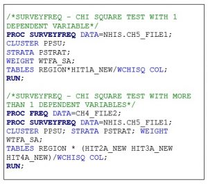
The independent (predictor or exposure) and dependent (outcome) variables are identified in each objective. PROC SURVEYFREQ is the procedure used to display the crosstabulation of variables and calculation of the chi square test result. You must add “/WCHISQ” at the end of the statement that begins with “tables.” You can calculate the chi square test for each dependent variable separately or you can run then together. You can enter the SAS syntax from Box 5.3 to determine the chi square test results.
Box 5.4. SAS SURVEY Procedure (PROC SURVEYFREQ with /WCHISQ) for running chi Square tests using 2018 NHIS Sample Adult analytic dataset
5.3.4 Survey Procedures for Logistic Regression
As stated in Chapter 4, crude and adjusted logistic regression models are used when the dependent (outcome) variable is binary/dichotomous.6 Crude and multivariable logistic regression models can be used to obtain results for research objective 5.5 in this chapter’s 2018 NHIS Sample Adult example. As a reminder:
- Objective 5.5: To determine the associations between sex (independent variable) and each HIT usage — looking up health information online, filling prescriptions, scheduling appointments, and communicating with a health care provider by e-mail — (dependent variables) before and after controlling for other contributing factors
The independent (predictor or exposure) and dependent (outcome) variables are identified in the objective. In this example, the contributing factors that will be controlled for to reduce bias are region and age. PROC SURVEYLOGISTIC is the procedure used to calculate the results after adjusting for the stratum, cluster and weight variables. You can enter the SAS syntax provided to determine the crude (Box 5.5) and multivariable (Box 5.6) results.
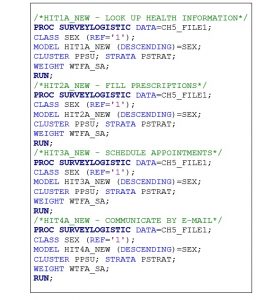
Box 5.5. SAS SURVEY procedure (PROC SURVEYLOGISTIC) for crude logistic regression results in the 2018 NHIS Sample Adult analytic dataset
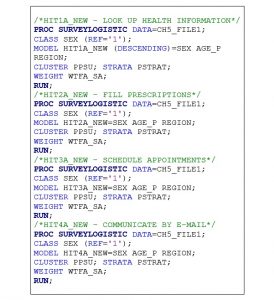
Box 5.6. SAS SURVEY procedure (PROC SURVEYLOGISTIC) for multivariable logistic regression results in the 2018 NHIS Sample Adult analytic dataset
The CLASS statement identifies the reference or comparison group for the categorical independent variable and other covariates. For the variable SEX, females will be compared to males. In the analytic dataset, males are represented by “1” and females are represented by “2.” Therefore, the reference category is “1” so that our results will represent the odds of females using HIT in comparison to males. The MODEL statement is set up as “dependent variable = independent variable (+ covariates for multivariable analysis).” The DESCENDING statement after the dependent variable identifies the higher value as the outcome of interest. For each HIT usage, “1=yes” will be the outcome that is modeled. Therefore, our results will indicate the odds of using health information technology instead of the odds of not using health information technology.
5.4 Summary
This chapter provided an overview of complex design features of national health surveys and how to run SAS SURVEY procedures to determine national estimates using primarily categorical data. The examples used in this chapter come from the 2018 NHIS Sample Adult public-use data files and focused on determining associations between demographic factors (region, sex) and HIT uses (look up health information, fill prescriptions, schedule appointments, and communicate with health care providers by e-mail) among US adults. SAS SURVEY procedures were demonstrated for running frequencies, means, chi square tests, and logistic regression models that account for the stratum, cluster, and weight variables.
5.5. References
- Lewis TH. Complex Survey Data Analysis with SAS. CRC Press, Taylor & Francis Group; 2017.
- Blewett LA, Dahlen HM, Spencer D, Rivera Drew JA, Lukanen E. Changes to the Design of the National Health Interview Survey to Support Enhanced Monitoring of Health Reform Impacts at the State Level. Am J Public Health. 2016;106(11):1961-1966. doi:10.2105/AJPH.2016.303430
- Finney Rutten LJ, Blake KD, Skolnick VG, Davis T, Moser RP, Hesse BW. Data Resource Profile: The National Cancer Institute’s Health Information National Trends Survey (HINTS). Int J Epidemiol. 2020;49(1):17-17j. doi:10.1093/ije/dyz083
- National Center for Health Statistics. National Health Interview Survey, 2011-2015. Public-use data file and documentation. Published August 5, 2020. Accessed August 10, 2020. https://www.cdc.gov/nchs/nhis/data-questionnaires-documentation.htm
- Parsons V, Moriarity C, Jonas K. Design and Estimation for the National Health Interview Survey, 2006–2015.; 2014:53. https://www.cdc.gov/nchs/data/series/sr_02/sr02_165.pdf
- Jacobsen KH. Introduction to Health Research Methods: A Practical Guide. 2nd ed. Jones & Bartlett Learning; 2017.
