4 Hydrometer Analysis

Introduction

The particle size distribution of soil containing a significant number of finer particles (silt and clay) cannot be performed by sieve analysis. The hydrometer analysis is a widely used method of obtaining an estimate of the distribution of soil particle sizes from the #200 (0.075 mm) sieve to around 0.001 mm.  The data are plotted on a semi-log plot of percent finer versus grain diameters to represent the particle size distribution. Both sieve analysis and hydrometer analysis are required to obtain the complete gradation curve of the coarse and fine fraction of many natural soils.

Practical Application

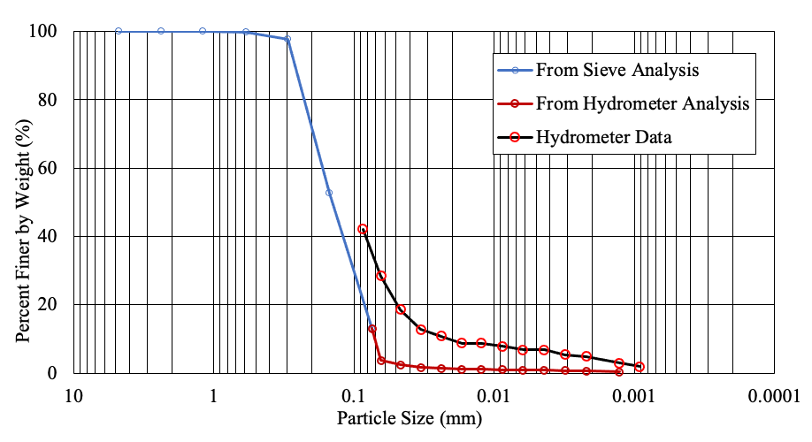
  • Hydrometer analysis is essential for obtaining the complete particle size distribution of such soils. Particle size distribution obtained from sieve analysis may be combined with the data from a hydrometer analysis to produce a complete gradation curve. It is possible to approximate the percentage of silt and clay particles present in the finer portion from the hydrometer analysis.
  • Particle size is one of the criteria used to determine whether a soil is suitable for building roads, embankments, dams, etc.
  • Information obtained from a particle size analysis can be used to predict soil-water movement if a permeability test is not available.

Objective

The objective of this experiment is:
  • To determine the particle size distribution of fine-grained soil (smaller than 0.075 mm diameter grains), using a hydrometer.

Equipment

  • Balance
  • Mixer (blender)
  • Hydrometer (152H model preferably,
  • Sedimentation cylinder (1000 mL cylinder)
  • Graduated 1000 mL cylinder for control jar
  • Dispersing agent [sodium hexametaphosphate (NaPO3) or sodium silicate (NaSiO3)]
  • Control cylinder
  • Thermometer
  • Beaker
  • Timing device

Standard Reference

  • ASTM D7928: Standard Test Method for Particle-Size Distribution (Gradation) of Fine-Grained Soils Using the Sedimentation (Hydrometer) Analysis

Method

  • Place 50 g of fine soil in a beaker, add 125 mL of the dispersing agent (sodium hexametaphosphate [40 g/L] solution) and stir the mixture until the soil is thoroughly wet. Let the soil soak for at least ten minutes.
    A person is pouring sodium hexametaphosphate solution from a glass flask into a mixing jar. Beside this there is a white container of sodium hexametaphosphate
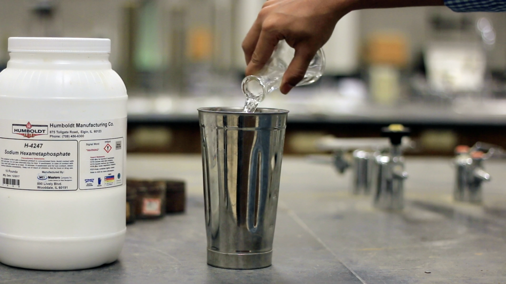
    Figure 4.1: Adding sodium hexametaphosphate solution
  • While the soil is soaking, add 125 mL of the dispersing agent to the control cylinder and fill it to the mark with distilled water. (The reading at the top of the meniscus formed by the hydrometer stem and the control solution is called the zero connection.) Record a reading less than zero as a negative (-) correction and a reading between zero and sixty as a positive (+) correction. The meniscus correction is the difference between the top of the meniscus and the level of the solution in the control jar (usually about +1). Shake the control cylinder to mix the contents thoroughly. Insert the hydrometer and thermometer into the control cylinder and note the zero correction and temperature, respectively.
    This image shows a reading of scale which is above zero. The scale is submerged in water into a glass jar.
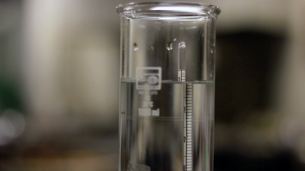
    Figure 4.2: Taking zero and meniscuscorrection reading
  • Transfer the soil slurry to a mixer by adding more distilled water, if necessary, until the mixing cup is at least half full. Then mix the solution for two minutes.
    A person a mixing soil slurry. He is holding the mixing jar close to the mixing machine.
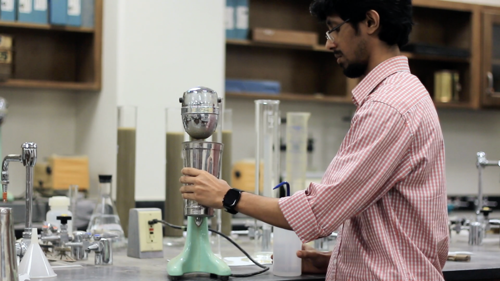
    Figure 4.3: Soil slurry preparation using a mixer
  • Immediately transfer the soil slurry into the empty sedimentation cylinder and add distilled water up to the mark.
  • Cover the open end of the cylinder with a stopper and secure it with the palm of your hand. Alternate turning the cylinder upside down and back upright for one minute, inverting it approximately 30 times.
    A person is pouring the soil slurry from the mixing jar to a glass jar. He is putting water into the jar for cleaning from a squeeze bottle at the same time.
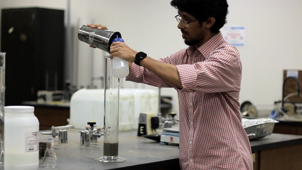
    Figure 4.4: Pouring the soil sample into the sedimentation cylinder
  • Set the cylinder down and record the time. Remove the stopper from the cylinder, and very slowly and carefully insert the hydrometer for the first reading. (Note: It should take about ten seconds to insert or remove the hydrometer to minimize any disturbance, and the release of the hydrometer should be made as close to the  reading depth as possible to avoid excessive bobbing.)
    Two glass jar placed side by side. Left glass jar is filled with water and soil mixture which has a scale submerged into it. Right glass jar has water like solution.
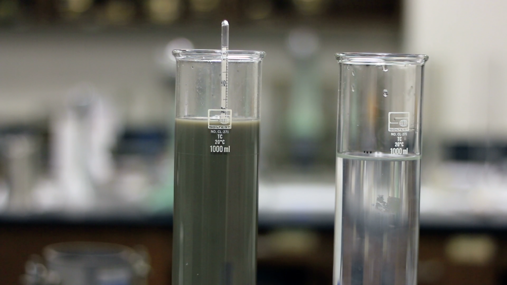
    Figure 4.5: Sedimentation cylinder and control cylinder during the hydrometer reading
  • Take the reading by observing the top of the meniscus that was formed by the suspension and the hydrometer stem. Remove the hydrometer slowly and place it back into the control cylinder. Very gently spin it in the control cylinder to remove any particles that may have adhered to it.
  • Take hydrometer readings at 15 sec, 30 sec, 1 min, 2 min, 4 min, 8 min, 15 min, 30 min, 1 hr., 2 hrs., 4 hrs., 8 hrs., 16 hrs., 24 hrs., and 48 hrs. These are approximate times that will usually give a satisfactory plot spread.
  • Record the temperature of the soil-water suspension to the nearest 0.5°C for each hydrometer reading.

Data Analysis

  • Apply the meniscus correction to the actual hydrometer reading.
  • Obtain the effective hydrometer depth (L in cm) for the corrected meniscus reading from Table 4-1.
  • Obtain the value of K from Table 4-2 if the Gs of the soil is known. If it is not known, assume that it is 2.65 for this purpose.
  •  Calculate the equivalent particle diameter by using the following formula:
    $D=K \times \sqrt{\frac{L}{t}}$
    Where t is given in minutes, and D is given in mm.
  • Determine the temperature correction CT from Table 4-3.
  • Determine correction factor “a” from Table 4-4 using Gs.
  • Calculate the corrected hydrometer reading as follows:
    Rc=RACTUAL– Zero Correction +CT
  • Calculate the percent finer as follows:
    $P=\frac{R_c \times a}{W_s} \times 100$
    Where, WS is the weight of the soil sample in grams.
  • Adjuste the percent fines as follows:
    $P_A=\frac{P\times F_{200}}{100}$
    Where, F200= % finer of #200 sieve as a percent
  • Plot the grain size curve D versus the adjusted percent finer on the semilogarithmic sheet.

Video Materials

Lecture Video

A PowerPoint presentation is created to understand the background and method of this experiment.

Demonstration Video

A short video is executed to demonstrate the experiment procedure and sample calculation.

Results and Discussions

Sample Data Sheet

Test date: September 15, 2002
Hydrometer Number: 152H
Specific Gravity of Soil: 2.56
% finer of #200 sieve as a percent, F200= 43.9%
Dispersing Agent: Sodium Hexametaphosphate
Weight of Soil Sample: 50.0 gm
Zero Correction: +6
Meniscus Correction: +1
Table 4.1: Values of effective depth based on hydrometer and sedimentation cylinder of specific sizes
For Hydrometer 151H
\begin{tabular}{|c|c|c|c|} \hline Corrected Hydrometer Reading & Effective Depth, L (cm) & Corrected Hydrometer Reading & Effective Depth, L (cm) \\ \hline 1.000 & 16.3 & 1.020 & 11.0 \\ \hline 1.001 & 16.0 & 1.021 & 10.7 \\ \hline 1.002 & 15.8 & 1.022 & 10.5 \\ \hline 1.003 & 15.5 & 1.023 & 10.2 \\ \hline 1.004 & 15.2 & 1.024 & 10.0 \\ \hline 1.005 & 15.0 & 1.025 & 9.7 \\ \hline 1.006 & 14.7 & 1.026 & 9.4 \\ \hline 1.007 & 14.4 & 1.027 & 9.2 \\ \hline 1.008 & 14.2 & 1.028 & 8.9 \\ \hline 1.009 & 13.9 & 1.029 & 8.6 \\ \hline 1.010 & 13.7 & 1.030 & 8.4 \\ \hline 1.011 & 13.4 & 1.031 & 8.1 \\ \hline 1.012 & 13.1 & 1.032 & 7.8 \\ \hline 1.013 & 12.9 & 1.033 & 7.6 \\ \hline 1.014 & 12.6 & 1.034 & 7.3 \\ \hline 1.015 & 12.3 & 1.035 & 7.0 \\ \hline 1.016 & 12.1 & 1.036 & 6.8 \\ \hline 1.017 & 11.8 & 1.037 & 6.5 \\ \hline 1.018 & 11.5 & 1.038 & 6.2 \\ \hline 1.019 & 11.3 & 1.039 & 5.9 \\ \hline \end{tabular}% }
For Hydrometer 152H
\begin{tabular}{|c|c|c|c|} \hline Corrected Hydrometer Reading & Effective Depth, L (cm) & Corrected Hydrometer Reading & Effective Depth, L (cm) \\ \hline 0 & 16.3 & 31 & 11.2 \\ \hline 1 & 16.1 & 32 & 11.1 \\ \hline 2 & 16.0 & 33 & 10.9 \\ \hline 3 & 15.8 & 34 & 10.7 \\ \hline 4 & 15.6 & 35 & 10.6 \\ \hline 5 & 15.5 & 36 & 10.4 \\ \hline 6 & 15.3 & 37 & 10.2 \\ \hline 7 & 15.2 & 38 & 10.1 \\ \hline 8 & 15.0 & 39 & 9.9 \\ \hline 9 & 14.8 & 40 & 9.7 \\ \hline 10 & 14.7 & 41 & 9.6 \\ \hline 11 & 14.5 & 42 & 9.4 \\ \hline 12 & 14.3 & 43 & 9.2 \\ \hline 13 & 14.2 & 44 & 9.1 \\ \hline 14 & 14.0 & 45 & 8.9 \\ \hline 15 & 13.8 & 46 & 8.8 \\ \hline 16 & 13.7 & 47 & 8.6 \\ \hline 17 & 13.5 & 48 & 8.4 \\ \hline 18 & 13.3 & 49 & 8.3 \\ \hline 19 & 13.2 & 50 & 8.1 \\ \hline 20 & 13.0 & 51 & 7.9 \\ \hline 21 & 12.9 & 52 & 7.8 \\ \hline 22 & 12.7 & 53 & 7.6 \\ \hline 23 & 12.5 & 54 & 7.4 \\ \hline 24 & 12.4 & 55 & 7.3 \\ \hline 25 & 12.2 & 56 & 7.1 \\ \hline 26 & 12.0 & 57 & 7.0 \\ \hline 27 & 11.9 & 58 & 6.8 \\ \hline 28 & 11.7 & 59 & 6.6 \\ \hline 29 & 11.5 & 60 & 6.5 \\ \hline 30 & 11.4 & & \\ \hline \end{tabular}% }
Table 4.2: Values of k for computing diameter of particle in hydrometer analysis
\begin{tabular}{|c|c|c|c|c|c|c|c|c|c|} \hline Temperature & \multicolumn{9}{c|}{Specific Gravity of Soil Particles} \\ \hline & 2.45 & 2.5 & 2.55 & 2.6 & 2.65 & 2.7 & 2.75 & 2.8 & 2.85 \\ \hline 16 & 0.0151 & 0.01505 & 0.01481 & 0.01457 & 0.01435 & 0.01414 & 0.01394 & 0.01374 & 0.01356 \\ \hline 17 & 0.01511 & 0.01486 & 0.01462 & 0.01439 & 0.01417 & 0.01396 & 0.01376 & 0.01356 & 0.01338 \\ \hline 18 & 0.01492 & 0.01467 & 0.01443 & 0.01421 & 0.01399 & 0.01378 & 0.01359 & 0.01339 & 0.01321 \\ \hline 19 & 0.01474 & 0.01449 & 0.01425 & 0.01403 & 0.01382 & 0.01361 & 0.01342 & 0.01323 & 0.01305 \\ \hline 20 & 0.01456 & 0.01431 & 0.01408 & 0.01386 & 0.01365 & 0.01344 & 0.01325 & 0.01307 & 0.01289 \\ \hline 21 & 0.01438 & 0.01414 & 0.01391 & 0.01369 & 0.01348 & 0.01328 & 0.01309 & 0.01291 & 0.01273 \\ \hline 22 & 0.01421 & 0.01397 & 0.01374 & 0.01353 & 0.01332 & 0.01312 & 0.01294 & 0.01276 & 0.01258 \\ \hline 23 & 0.01404 & 0.01381 & 0.01358 & 0.01337 & 0.01317 & 0.01297 & 0.01279 & 0.01261 & 0.01243 \\ \hline 24 & 0.01388 & 0.01365 & 0.01342 & 0.01321 & 0.01301 & 0.01282 & 0.01264 & 0.01246 & 0.01229 \\ \hline 25 & 0.01372 & 0.01349 & 0.01327 & 0.01306 & 0.01286 & 0.01267 & 0.01249 & 0.01232 & 0.01215 \\ \hline 26 & 0.01357 & 0.01334 & 0.01312 & 0.01291 & 0.01272 & 0.01253 & 0.01235 & 0.01218 & 0.01201 \\ \hline 27 & 0.01342 & 0.01319 & 0.01297 & 0.01277 & 0.01258 & 0.01239 & 0.01221 & 0.01204 & 0.01188 \\ \hline 28 & 0.01327 & 0.01304 & 0.01283 & 0.01264 & 0.01244 & 0.01255 & 0.01208 & 0.01191 & 0.01175 \\ \hline 29 & 0.01312 & 0.0129 & 0.01269 & 0.01249 & 0.0123 & 0.01212 & 0.01195 & 0.01178 & 0.01162 \\ \hline 30 & 0.01298 & 0.01276 & 0.01256 & 0.01236 & 0.01217 & 0.01199 & 0.01182 & 0.01165 & 0.01149 \\ \hline \end{tabular}% }
Table 4.3: Temperature correction factors, CT
\begin{tabular}{|c|c|} \hline Temperature (°C) & factor (CT) \\ \hline 15 & 1.10 \\ \hline 16 & -0.90 \\ \hline 17 & -0.70 \\ \hline 18 & -0.50 \\ \hline 19 & -0.30 \\ \hline 20 & 0.00 \\ \hline 21 & 0.20 \\ \hline 22 & 0.40 \\ \hline 23 & 0.70 \\ \hline 24 & 1.00 \\ \hline 25 & 1.30 \\ \hline 26 & 1.65 \\ \hline 27 & 2.00 \\ \hline 28 & 2.50 \\ \hline 29 & 3.05 \\ \hline 30 & 3.80 \\ \hline \end{tabular}% }
Table 4.4: Correction factors a for unit weight of solids
\begin{tabular}{|c|c|} \hline Unit Weight of Soil Solids, g/cm3 & Correction factor, a \\ \hline 2.85 & 0.96 \\ \hline 2.8 & 0.97 \\ \hline 2.75 & 0.98 \\ \hline 2.7 & 0.99 \\ \hline 2.65 & 1 \\ \hline 2.6 & 1.01 \\ \hline 2.55 & 1.02 \\ \hline 2.5 & 1.04 \\ \hline \end{tabular}% }
Sample Data Sheet
\resizebox{\linewidth}{% \begin{tabular}{|c|c|c|c|c|c|c|c|c|c|c|c|c|c|} \hline Date & Time & Elapsed & Temp & Actual & Hydr. Corr. & L & K from & D mm & $C_T$ & a from & Corr. & \% & \% \\ & & Time (min) & & Hydr. & for & from & Table & & from & Table & Hydr. & Finer, & Adjusted \\ & & & & Rdg. & Meniscus & Table & 4.2 & & Table & 4.4 & Rdg. & P & Finer, \\ & & & & $R_a$ & & 4.1 & & & 4.3 & & $R_c$ & & $P_A$ \\ \hline 15-Sep & 4:06 PM & 0 & 25 & 55 & 56 & 7.1 & 0.01326 & 0 & 1.3 & 1.018 & - & - & - \\ \hline & 4:07 & 1 & 25 & 47 & 48 & 8.4 & 0.01326 & 0.03029 & 1.3 & 1.018 & 42.3 & 86.1 & 37.8 \\ \hline & 4:08 & 2 & 25 & 42 & 43 & 9.2 & 0.01326 & 0.02844 & 1.3 & 1.018 & 37.3 & 75.9 & 33.3 \\ \hline & 4:10 & 4 & 25 & 40 & 41 & 9.6 & 0.01326 & 0.02054 & 1.3 & 1.018 & 35.3 & 71.9 & 31.6 \\ \hline & 4:14 & 8 & 25 & 37 & 38 & 10.1 & 0.01326 & 0.01490 & 1.3 & 1.018 & 32.3 & 65.8 & 28.6 \\ \hline & 4:22 & 16 & 25 & 32 & 33 & 10.9 & 0.01326 & 0.01094 & 1.3 & 1.018 & 27.3 & 55.6 & 24.1 \\ \hline & 4:40 & 34 & 25 & 28 & 29 & 11.5 & 0.01326 & 0.00771 & 1.3 & 1.018 & 23.3 & 47.4 & 20.8 \\ \hline & 6:22 & 136 & 23 & 22 & 23 & 12.5 & 0.01356 & 0.00411 & 0.7 & 1.018 & 16.7 & 34 & 14.9 \\ \hline 16-Sep & 5:24 PM & 1518 & 22 & 15 & 16 & 13.7 & 0.01366 & 0.00130 & 0.4 & 1.018 & 9.4 & 19.1 & 8.4 \\ \hline \end{tabular}% }
A semi-log graph where x-axis is particle size in millimeter and y-axis is percent finer weight in %. This graph has three lines. Blue one with small circle is from sieve analysis. Red one with small circle is from hydrometer analysis and red one with larger circle is the hydrometer data. X-axis ranges from 10 to 0.001 and y-axis ranges from 0 to 100.
Figure 4.6: A typical grain-size distribution curve (From sieve and hydrometer analysis)

Blank Data Sheet

Test date:
Hydrometer Number:
Specific Gravity of Soil:
% finer of #200 sieve as a percent, F200:
Dispersing Agent:
Weight of Soil Sample:
Zero Correction:
Meniscus Correction:
\resizebox{\textwidth}{% \begin{tabular}{|c|c|c|c|c|c|c|c|c|c|c|c|c|c|} \hline Date & Time & Elapsed & Temp & Actual & Hydr. Corr. & L & K from & D mm & $C_T$ & a from & Corr. & \% & \% \\ & & Time & & Hydr. & for & from & Table & & from & Table & Hydr. & Finer, & Adjusted \\ & & (min) & & Rdg. & Meniscus & Table & 4.2 & & Table & 4.4 & Rdg. & P & Finer, \\ & & & & $R_a$ & & 4.1 & & & 4.3 & & $R_c$ & & $P_A$ \\ \hline & & & & & & & & & & & & & \\ \hline & & & & & & & & & & & & & \\ \hline & & & & & & & & & & & & & \\ \hline & & & & & & & & & & & & & \\ \hline & & & & & & & & & & & & & \\ \hline & & & & & & & & & & & & & \\ \hline & & & & & & & & & & & & & \\ \hline & & & & & & & & & & & & & \\ \hline & & & & & & & & & & & & & \\ \hline \end{tabular}% }

Report

Use the template provided to prepare your lab report for this experiment. Your report should include the following:
  • Objective of the test
  • Applications of the test
  • Apparatus used
  • Test procedures (optional)
  • Analysis of the test results – Complete the table provided and show one sample calculation. Draw the grain size distribution curve for the data from the hydrometer analysis only and the combined grain-size distribution curve.
  • Summary and conclusions – Comment on the shape of grain size distribution curve of the given soil sample

License

Icon for the Creative Commons Attribution-NonCommercial 4.0 International License

Properties and Behavior of Soil - Online Lab Manual Copyright © 2021 by MD Sahadat Hossain, Ph.D., P.E.; Md Azijul Islam; Faria Fahim Badhon; and Tanvir Imtiaz is licensed under a Creative Commons Attribution-NonCommercial 4.0 International License, except where otherwise noted.

Share This Book