Experiment #10: Pumps
1. Introduction
In waterworks and wastewater systems, pumps are commonly installed at the source to raise the water level and at intermediate points to boost the water pressure. The components and design of a pumping station are vital to its effectiveness. Centrifugal pumps are most often used in water and wastewater systems, making it important to learn how they work and how to design them. Centrifugal pumps have several advantages over other types of pumps, including:
- Simplicity of construction – no valves, no piston rings, etc.;
- High efficiency;
- Ability to operate against a variable head;
- Suitable for being driven from high-speed prime movers such as turbines, electric motors, internal combustion engines etc.; and
- Continuous discharge.
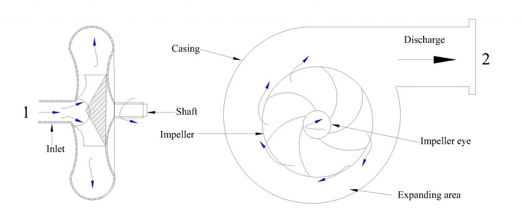
A centrifugal pump consists of a rotating shaft that is connected to an impeller, which is usually comprised of curved blades. The impeller rotates within its casing and sucks the fluid through the eye of the casing (point 1 in Figure 10.1). The fluid’s kinetic energy increases due to the energy added by the impeller and enters the discharge end of the casing that has an expanding area (point 2 in Figure 10.1). The pressure within the fluid increases accordingly.
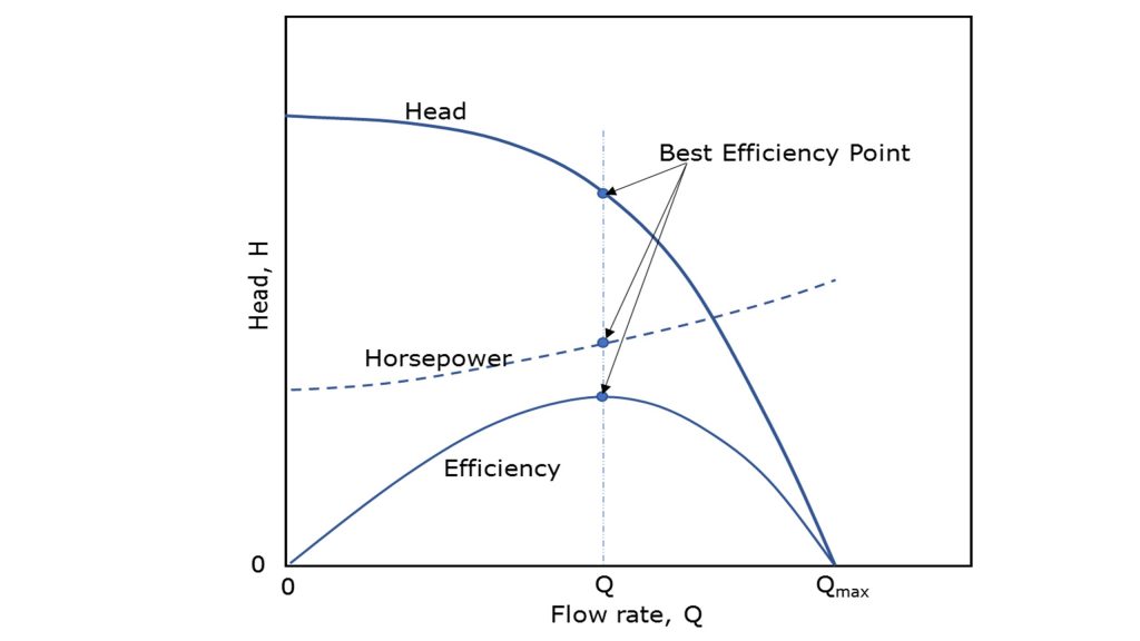
The performance of a centrifugal pump is presented as characteristic curves in Figure 10.2, and is comprised of the following:
- Pumping head versus discharge,
- Brake horsepower (input power) versus discharge, and
- Efficiency versus discharge.
The characteristic curves of commercial pumps are provided by manufacturers. Otherwise, a pump should be tested in the laboratory, under various discharge and head conditions, to produce such curves. If a single pump is incapable of delivering the design flow rate and pressure, additional pumps, in series or parallel with the original pump, can be considered. The characteristic curves of pumps in series or parallel should be constructed since this information helps engineers select the types of pumps needed and how they should be configured.
2. Practical Application
Many pumps are in use around the world to handle liquids, gases, or liquid-solid mixtures. There are pumps in cars, swimming pools, boats, water treatment facilities, water wells, etc. Centrifugal pumps are commonly used in water, sewage, petroleum, and petrochemical pumping. It is important to select the pump that will best serve the project’s needs.
3. Objective
The objective of this experiment is to determine the operational characteristics of two centrifugal pumps when they are configured as a single pump, two pumps in series, and two pumps in parallel.
4. Method
Each configuration (single pump, two pumps in series, and two pumps in parallel) will be tested at pump speeds of 60, 70, and 80 rev/sec. For each speed, the bench regulating valve will be set to fully closed, 25%, 50%, 75%, and 100% open. Timed water collections will be performed to determine flow rates for each test, and the head, hydraulic power, and overall efficiency ratings will be obtained.
5. Equipment
The following equipment is required to perform the pumps experiment:
- P6100 hydraulics bench, and
- Stopwatch.
6. Equipment Description
The hydraulics bench is fitted with a single centrifugal pump that is driven by a single-phase A.C. motor and controlled by a speed control unit. An auxiliary pump and the speed control unit are supplied to enhance the output of the bench so that experiments can be conducted with the pumps connected either in series or in parallel. Pressure gauges are installed at the inlet and outlet of the pumps to measure the pressure head before and after each pump. A watt-meter unit is used to measure the pumps’ input electrical power [10].
7. Theory
7.1. General Pump Theory
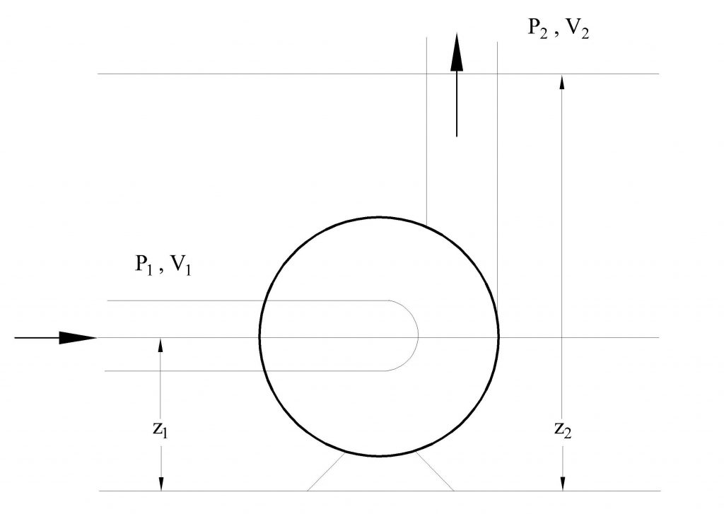
Consider the pump shown in Figure 10.3. The work done by the pump, per unit mass of fluid, will result in increases in the pressure head, velocity head, and potential head of the fluid between points 1 and 2. Therefore:
- work done by pump per unit mass = W/M
- increase in pressure head per unit mass

- increase in velocity head per unit mass

- increase in potential head per unit mass

in which:
W: work
M: mass
P: pressure
 : density
v: flow velocity
g: acceleration due to gravity
z: elevation
Applying Bernoulli’s equation between points 1 and 2 in Figure 10.3 results in:

Since the difference between elevations and velocities at points 1 and 2 are negligible, the equation becomes:

Dividing both sides of this equation by gives:

The right side of this equation is the manometric pressure head, Hm, therefore:

7.2. Power and Efficiency
The hydraulic power (Wh) supplied to the fluid by the pump is the product of the pressure increase and the flow rate:

The pressure increase produced by the pump can be expressed in terms of the manometric head,

Therefore:

The overall efficiency ( ) of the pump-motor unit can be determined by dividing the hydraulic power (Wh) by the input electrical power (Wi), i.e.:

7.3. Single Pump – Pipe System performance
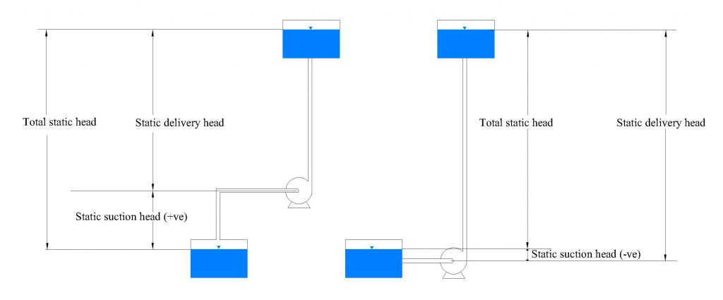
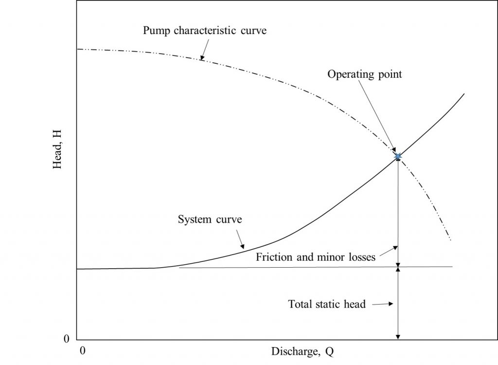
While pumping fluid, the pump has to overcome the pressure loss that is caused by friction in any valves, pipes, and fittings in the pipe system. This frictional head loss is approximately proportional to the square of the flow rate. The total system head that the pump has to overcome is the sum of the total static head and the frictional head. The total static head is the sum of the static suction lift and the static discharge head, which is equal to the difference between the water levels of the discharge and the source tank (Figure 10.4). A plot of the total head-discharge for a pipe system is called a system curve; it is superimposed onto a pump characteristic curve in Figure 10.5. The operating point for the pump-pipe system combination occurs where the two graphs intercept [10].
7.4. Pumps in Series
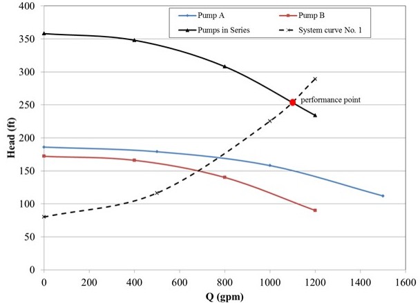
Pumps are used in series in a system where substantial head changes take place without any appreciable difference in discharge. When two or more pumps are configured in series, the flow rate throughout the pumps remains the same; however, each pump contributes to the increase in the head so that the overall head is equal to the sum of the contributions of each pump [10]. For n pumps in series:


The composite characteristic curve of pumps in series can be prepared by adding the ordinates (heads) of all of the pumps for the same values of discharge. The intersection point of the composite head characteristic curve and the system curve provides the operating conditions (performance point) of the pumps (Figure 10.6).
7.5. Pumps in Parallel
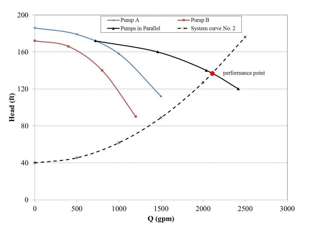
Parallel pumps are useful for systems with considerable discharge variations and with no appreciable head change. In parallel, each pump has the same head. However, each pump contributes to the discharge so that the total discharge is equal to the sum of the contributions of each pump [10]. Thus for pumps:


The composite head characteristic curve is obtained by summing up the discharge of all pumps for the same values of head. A typical pipe system curve and performance point of the pumps are shown in Figure 10.7.
8. Experimental Procedure
8.1. Experiment 1: Characteristics of a Single Pump
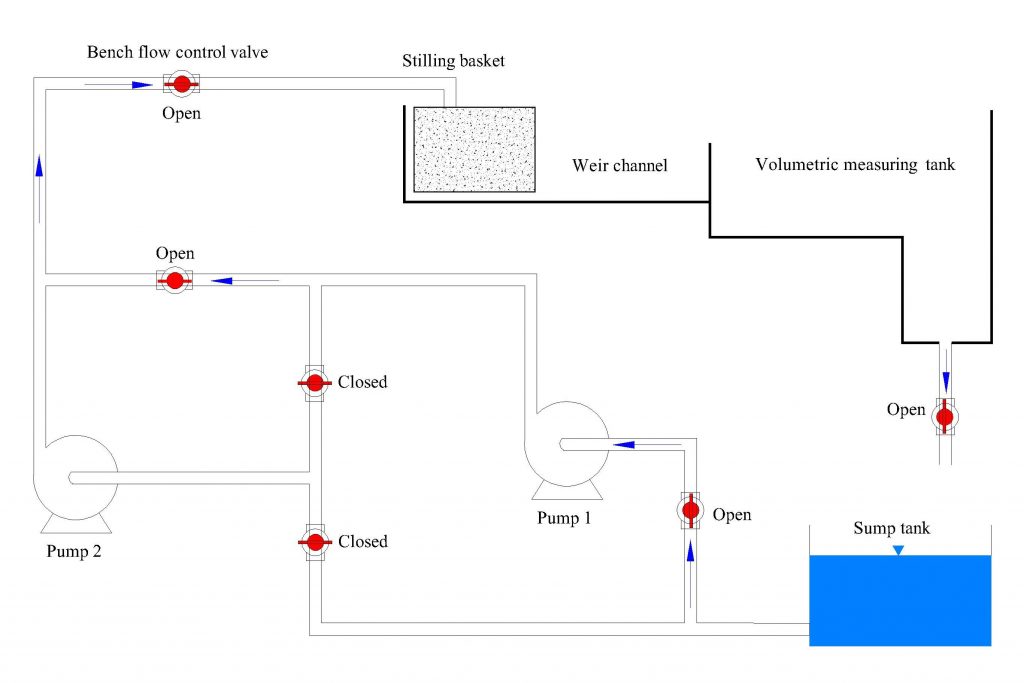
a) Set up the hydraulics bench valves, as shown in Figure 10.8, to perform the single pump test.
b) Start pump 1, and increase the speed until the pump is operating at 60 rev/sec.
c) Turn the bench regulating valve to the fully closed position.
d) Record the pump 1 inlet pressure (P1) and outlet pressure (P2). Record the input power from the watt-meter (Wi). (With the regulating valve fully closed, discharge will be zero.)
e) Repeat steps (c) and (d) by setting the bench regulating valve to 25%, 50%, 75%, and 100% open.
f) For each control valve position, measure the flow rate by either collecting a suitable volume of water (a minimum of 10 liters) in the measuring tank, or by using the rotameter.
g) Increase the speed until the pump is operating at 70 rev/sec and 80 rev/sec, and repeat steps (c) to (f) for each speed.
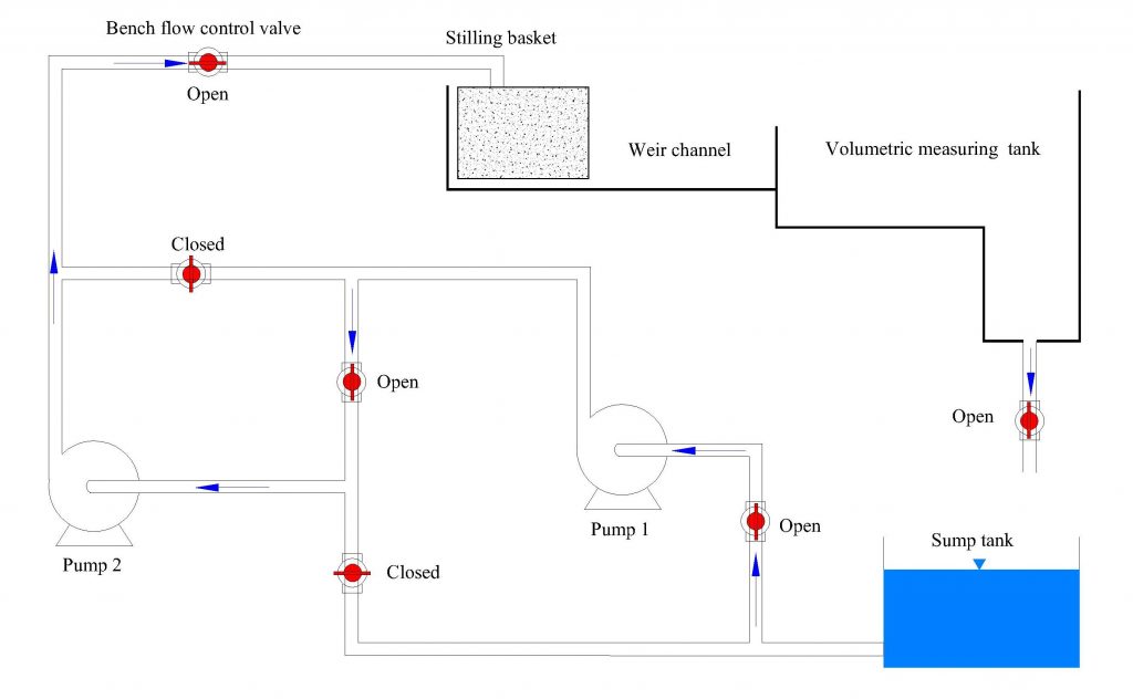
8.2. Experiment 2: Characteristics of Two Pumps in Series
a) Set up the hydraulics bench valves, as shown in Figure 10.9, to perform the two pumps in series test.
b) Start pumps 1 and 2, and increase the speed until the pumps are operating at 60 rev/sec.
c) Turn the bench regulating valve to the fully closed position.
d) Record the pump 1 and 2 inlet pressure (P1) and outlet pressure (P2). Record the input power for pump 1 from the wattmeter (Wi). (With the regulating valve fully closed, discharge will be zero.)
e) Repeat steps (c) and (d) by setting the bench regulating valve to 25%, 50%, 75%, and 100% open.
f) For each control valve position, measure the flow rate by either collecting a suitable volume of water (a minimum of 10 liters) in the measuring tank, or by using the rotameter.
g) Increase the speed until the pump is operating at 70 rev/sec and 80 rev/sec, and repeat steps (c) to (f) for each speed.
Note: Wattmeter readings should be recorded for both pumps, assuming that both pumps have the same input power.
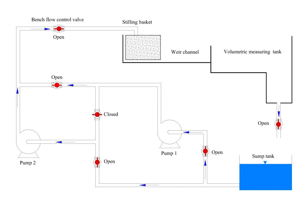
8.3. Experiment 3: Characteristics of Two Pumps in Parallel
a) Configure the hydraulic bench, as shown in Figure 10.10, to conduct the test for pumps in parallel.
b) Repeat steps (b) to (g) in Experiment 2.
9. Results and Calculations
Please visit this link for accessing excel workbook of this manual.
9.1. Result
Record your measurements for Experiments 1 to 3 in the Raw Data Tables.
Raw Data Table
| Single Pump: 60 rev/s | |||||
| Valve Open Position | 0% | 25% | 50% | 75% | 100% |
| Volume (L) | |||||
| Time (s) | |||||
| Pump 1 Inlet Pressure, P1 (bar) | |||||
| Pump 1 Outlet Pressure, P2 (bar) | |||||
| Pump 1 Electrical Input Power (Wi) | |||||
| Single Pump: 70 rev/s | |||||
| Valve Open Position | 0% | 25% | 50% | 75% | 100% |
| Volume (L) | |||||
| Time (s) | |||||
| Pump 1 Inlet Pressure, P1 (bar) | |||||
| Pump 1 Outlet Pressure, P2 (bar) | |||||
| Pump 1 Electrical Input Power (Wi) | |||||
| Single Pump: 80 rev/s | |||||
| Valve Open Position | 0% | 25% | 50% | 75% | 100% |
| Volume (L) | |||||
| Time (s) | |||||
| Pump 1 Inlet Pressure, P1 (bar) | |||||
| Pump 1 Outlet Pressure, P2 (bar) | |||||
| Pump 1 Electrical Input Power (Wi) | |||||
| Two Pumps in Series: 60 rev/s | |||||
| Valve Open Position | 0% | 25% | 50% | 75% | 100% |
| Volume (L) | |||||
| Time (s) | |||||
| Pump 1 Inlet Pressure, P1 (bar) | |||||
| Pump 1 Outlet Pressure, P2 (bar) | |||||
| Pump 1 Electrical Input Power (Wi) | |||||
| Pump 2 Inlet Pressure, P1 (bar) | |||||
| Pump 2 Outlet Pressure, P2 (bar) | |||||
| Pump 2 Electrical Input Power (Wi) | |||||
| Two Pumps in Series: 70 rev/s | |||||
| Valve Open Position | 0% | 25% | 50% | 75% | 100% |
| Volume (L) | |||||
| Time (s) | |||||
| Pump 1 Inlet Pressure, P1 (bar) | |||||
| Pump 1 Outlet Pressure, P2 (bar) | |||||
| Pump 1 Electrical Input Power (Wi) | |||||
| Pump 2 Inlet Pressure, P1 (bar) | |||||
| Pump 2 Outlet Pressure, P2 (bar) | |||||
| Pump 2 Electrical Input Power (Wi) | |||||
| Two Pumps in Series: 80 rev/s | |||||
| Valve Open Position | 0% | 25% | 50% | 75% | 100% |
| Volume (L) | |||||
| Time (s) | |||||
| Pump 1 Inlet Pressure, P1 (bar) | |||||
| Pump 1 Outlet Pressure, P2 (bar) | |||||
| Pump 1 Electrical Input Power (Wi) | |||||
| Pump 2 Inlet Pressure, P1 (bar) | |||||
| Pump 2 Outlet Pressure, P2 (bar) | |||||
| Pump 2 Electrical Input Power (Wi) | |||||
| Two Pumps in Parallel: 60 rev/s | |||||
| Valve Open Position | 0% | 25% | 50% | 75% | 100% |
| Volume (L) | |||||
| Time (s) | |||||
| Pump 1 Inlet Pressure, P1 (bar) | |||||
| Pump 1 Outlet Pressure, P2 (bar) | |||||
| Pump 1 Electrical Input Power (Wi) | |||||
| Pump 2 Inlet Pressure, P1 (bar) | |||||
| Pump 2 Outlet Pressure, P2 (bar) | |||||
| Pump 2 Electrical Input Power (Wi) | |||||
| Two Pumps in Parallel: 70 rev/s | |||||
| Valve Open Position | 0% | 25% | 50% | 75% | 100% |
| Volume (L) | |||||
| Time (s) | |||||
| Pump 1 Inlet Pressure, P1 (bar) | |||||
| Pump 1 Outlet Pressure, P2 (bar) | |||||
| Pump 1 Electrical Input Power (Wi) | |||||
| Pump 2 Inlet Pressure, P1 (bar) | |||||
| Pump 2 Outlet Pressure, P2 (bar) | |||||
| Pump 2 Electrical Input Power (Wi) | |||||
| Two Pumps in Parallel: 80 rev/s | |||||
| Valve Open Position | 0% | 25% | 50% | 75% | 100% |
| Volume (L) | |||||
| Time (s) | |||||
| Pump 1 Inlet Pressure, P1 (bar) | |||||
| Pump 1 Outlet Pressure, P2 (bar) | |||||
| Pump 1 Electrical Input Power (Wi) | |||||
| Pump 2 Inlet Pressure, P1 (bar) | |||||
| Pump 2 Outlet Pressure, P2 (bar) | |||||
| Pump 2 Electrical Input Power (Wi) | |||||
9.2. Calculations
- If the volumetric measuring tank was used, then calculate the flow rate from:

- Correct the pressure rise measurement (outlet pressure) across the pump by adding a 0.07 bar to allow for the difference of 0.714 m in height between the measurement point for the pump outlet pressure and the actual pump outlet connection.
- Convert the pressure readings from bar to N/m2 (1 Bar=105 N/m2), then calculate the manometric head from:

- Calculate the hydraulic power (in watts) from Equation 6 where Q is in m3/s, in kg/m3, g in m/s2, and Hm in meter.
- Calculate the overall efficiency from Equation 7.
Note:
– Overall head for pumps in series is calculated using Equation 8b.
– Overall head for pumps in parallel is calculated using Equation 9b.
– Overall electrical input power for pumps in series and in parallel combination is equal to (Wi)pump1+(Wi)pump2.
- Summarize your calculations in the Results Tables.
Result Tables
| Single Pump: N (rev/s) | |||||
| Valve Open Position | 0% | 25% | 50% | 75% | 100% |
| Flow Rate, Q (L/min) | |||||
| Flow Rate, Q (m3/s) | |||||
| Pump 1 Inlet Pressure, P1 (N/m2) | |||||
| Pump 1 Outlet Corrected Pressure, P2 (N/m2) | |||||
| Pump 1 Electrical Input Power (Watts) | |||||
| Pump 1 Head, Hm (m) | |||||
| Pump 1 Hydraulic Power, Wh (Watts) | |||||
| Pump 1 Overall Efficiency, η0 (%) | |||||
| Two Pumps in Series: N (rev/s) | |||||
| Valve Open Position | 0% | 25% | 50% | 75% | 100% |
| Flow Rate, Q (L/min) | |||||
| Flow Rate, Q (m3/s) | |||||
| Pump 1 Inlet Pressure, P1 (N/m2) | |||||
| Pump 1 Outlet Corrected Pressure, P2 (N/m2) | |||||
| Pump 1 Electrical Input Power (Watts) | |||||
| Pump 2 Inlet Pressure, P1 (N/m2) | |||||
| Pump 2 Outlet Corrected Pressure, P2 (N/m2) | |||||
| Pump 2 Electrical Input Power (Watts) | |||||
| Pump 1 Head, Hm (m) | |||||
| Pump 1 Hydraulic Power, Wh (Watts) | |||||
| Pump 2 Head, Hm (m) | |||||
| Pump 2 Hydraulic Power, Wh (Watts) |
|||||
| Overall Head, Hm (m) | |||||
| Overall Hydraulic Power, Wh (Watts) | |||||
| Overall Electrical Input Power, Wi (Watts) | |||||
| Both Pumps Overall Efficiency, η0 (%) | |||||
| Two Pumps in Parallel: N (rev/s) | |||||
| Valve Open Position | 0% | 25% | 50% | 75% | 100% |
| Flow Rate, Q (L/min) | |||||
| Flow Rate, Q (m3/s) | |||||
| Pump 1 Inlet Pressure, P1 (N/m2) | |||||
| Pump 1 Outlet Corrected Pressure, P2 (N/m2) | |||||
| Pump 1 Electrical Input Power (Watts) | |||||
| Pump 2 Inlet Pressure, P1 (N/m2) | |||||
| Pump 2 Outlet Corrected Pressure, P2 (N/m2) | |||||
| Pump 2 Electrical Input Power (Watts) | |||||
| Pump 1 Head, Hm (m) | |||||
| Pump 1 Hydraulic Power, Wh (Watts) | |||||
| Pump 2 Head, Hm (m) | |||||
| Pump 2 Hydraulic Power, Wh (Watts) |
|||||
| Overall Head, Hm (m) | |||||
| Overall Hydraulic Power, Wh (Watts) | |||||
| Overall Electrical Input Power, Wi (Watts) | |||||
| Both Pumps Overall Efficiency, η0 (%) | |||||
10. Report
Use the template provided to prepare your lab report for this experiment. Your report should include the following:
- Table(s) of raw data
- Table(s) of results
- Graph(s)
- Plot head in meters as y-axis against volumetric flow, in liters/min as x-axis.
- Plot hydraulic power in watts as y-axis against volumetric flow, in liters/min as x-axis.
- Plot efficiency in % as y-axis against volumetric flow, in liters/min as x-axis on your graphs.
In each of above graphs, show the results for single pump, two pumps in series, and two pumps in parallel – a total of three graphs. Do not connect the experimental data points, and use best fit to plot the graphs
- Discuss your observations and any sources of error in preparation of pump characteristics.
