Chapter 5: Motion and Forces
This chapter discusses the basic elements of accelerated motion and motion at constant speed to help estimate braking distance and safe travel speeds. Concepts of motion along a straight line are also helpful in estimating headways and flow rates on the facilities. Accelerated motion along a circular path provides a conceptual understanding of roadway superelevation (or banking; also see Chapter 6).
This chapter also describes forces acting on static objects. An understanding of friction forces and normal reactions is critical to transportation infrastructure design. The gravity model is useful as a prerequisite to understanding the dynamics of travel demand (trip distribution between traffic analysis zones (TAZs)).
Learning Objectives
At the end of the chapter, the reader should be able to do the following:
- Describe the gravity model.
- Estimate the friction force and Normal Reaction on a static object.
- Describe the motion of an object in the graphic form through the time-space diagram.
- Use kinematic equations to solve for displacement, time, velocity, and acceleration of an object.
- Describe the motion of an object along a circular path.
- Identify topics in the introductory transportation engineering courses that build on the concepts discussed in this chapter.
Units and Measurements
Physical Quantities and Units
We define a physical quantity either by specifying how it is measured or by stating how it is calculated from other measurements. For example, we define distance and time by specifying methods for measuring them, whereas we define average speed by stating that it is calculated as distance traveled divided by time of travel.
Measurements of physical quantities are expressed in terms of units, which are standardized values. For example, the length of a race, which is a physical quantity, can be expressed in units of meters (for sprinters) or kilometers (for distance runners). Without standardized units, it would be extremely difficult for scientists to express and compare measured values in a meaningful way.
There are two major systems of units used in the world: SI units (also known as the metric system) and English units (also known as the customary or imperial system). English units were historically used in nations once ruled by the British Empire and are still widely used in the United States. Virtually every other country in the world now uses SI units as the standard; the metric system is also the standard system agreed upon by scientists and mathematicians. The acronym “SI” is derived from the French Système International.
SI Units of Time, Length, and Mass
SI units are part of the metric system. Metric systems have the advantage that conversions of units involve base-10 number system. There are 100 centimeters in a meter, 1000 meters in a kilometer, and so on. In nonmetric systems, such as the system of U.S. customary units, the relationships are not as simple—there are 12 inches in a foot, 5280 feet in a mile, and so on.
| Length | Mass | Time |
|---|---|---|
| Meter (m) | Kilogram (kg) | Second (s) |
It is often necessary to convert from one type of unit to another. Let us consider a simple example of how to convert units. Let us say that we want to convert 80 meters (m) to kilometers (km). The first thing to do is to list the units that you have and the units that you want to convert to. In this case, we have units in meters, and we want to convert to kilometers.
Next, we need to determine a conversion factor relating meters to kilometers. A conversion factor is a ratio expressing how many of one unit are equal to another unit. For example, there are 12 inches in 1 foot, 100 centimeters in 1 meter, 60 seconds in 1 minute, and so on. In this case, we know that there are 1,000 meters in 1 kilometer.
Now we can set up our unit conversion. We will write the units that we have and then multiply them by the conversion factor so that the units cancel out, as shown:
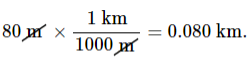
Note that the “m” unit cancels, leaving only the desired “km” unit. You can use this method to convert between any types of units.
Displacement
Position:
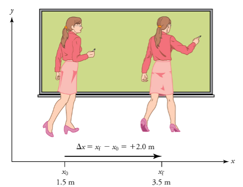
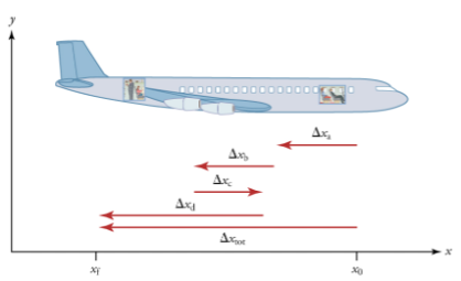
To describe the motion of an object, you must first be able to describe its position—where it is at any particular time. More precisely, you need to specify its position relative to a convenient reference frame. Earth is often used as a reference frame, and we often describe the position of an object as it relates to stationary objects in that reference frame. For example, a rocket launch would be described in terms of the position of the rocket with respect to the Earth as a whole, while a professor’s position could be described in terms of where she is in relation to the nearby white board. (See Figure 1). In other cases, we use reference frames that are not stationary but are in motion relative to the Earth. To describe the position of a person in an airplane, for example, we use the airplane, not the Earth, as the reference frame. (See Figure 2).
 displacement of the professor relative to the blackboard is represented by an arrow pointing to the right.
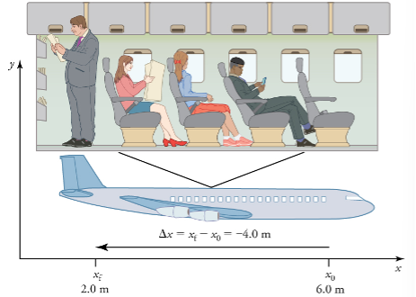
Displacement:
If an object moves relative to a reference frame (for example, if a professor moves to the right relative to a white board or a passenger moves toward the rear of an airplane), then the object’s position changes. This change in position is known as displacement. The word “displacement” implies that an object has moved or has been displaced.
Displacement is the change in position of an object:

Where  is displacement,
  is the final position, and
  is the initial position.
The Greek letter  (delta) means “change in” whatever quantity follows it; thus, means change in position. Always solve for displacement by subtracting initial position from final position .
Note that the SI unit for displacement is the meter (m), but sometimes kilometers, miles, feet, and other units of length are used. Keep in mind that when units other than the meter are used in a problem, you may need to convert them into meters to complete the calculation.
Note that displacement has a direction as well as a magnitude. The professor’s displacement is 2.0 m to the right, and the airline passenger’s displacement is 4.0 m toward the rear. In one-dimensional motion, direction can be specified with a plus or minus sign. When you begin a problem, you should select which direction is positive (usually that will be to the right or up, but you are free to select positive as being any direction). The professor’s initial position is  and her final position is
  . Thus, her displacement is

In this coordinate system, motion to the right is positive, whereas motion to the left is negative. Similarly, the airplane passenger’s initial position is  and his final position is
  so his displacement is

His displacement is negative because his motion is toward the rear of the plane, or in the negative x direction in our coordinate system.
Distance
Although displacement is described in terms of direction, distance is not. Distance is defined to be the magnitude or size of displacement between two positions. Note that the distance between two positions is different from the distance traveled between them. Distance traveled is the total length of the path traveled between two positions. Distance has no direction and, thus, no sign. For example, the distance the professor walks is 2.0 m. The distance the airplane passenger walks is 4.0 m.
Check Your Understanding: Displacement
Vectors, Scalars, and Coordinate Systems
What is the difference between distance and displacement? Whereas displacement is defined by both direction and magnitude, distance is defined only by magnitude. Displacement is an example of a vector quantity. Distance is an example of a scalar quantity. A vector is any quantity with both magnitude and direction. Other examples of vectors include a velocity of 90 km/h east and a force of 500 newtons straight down.
The direction of a vector in one-dimensional motion is given simply by a plus (+) or minus (−) sign. Vectors are represented graphically by arrows. An arrow used to represent a vector has a length proportional to the vector’s magnitude (e.g., the larger the magnitude, the longer the length of the vector) and points in the same direction as the vector.
Some physical quantities, like distance, either have no direction or none is specified. A scalar is any quantity that has a magnitude, but no direction. For example, a  temperature, the 250 kilocalories (250 Calories) of energy in a candy bar, a 90 km/h speed limit, a person’s 1.8 m height, and a distance of 2.0 m are all scalars – quantities with no specified direction. Note, however, that a scalar can be negative, such as
  temperature. In this case, the minus sign indicates a point on a scale rather than a direction. Scalars are never represented by arrows.
Coordinate Systems for One-Dimensional Motion
To describe the direction of a vector quantity, you must designate a coordinate system within the reference frame. For one-dimensional motion, this is a simple coordinate system consisting of a one-dimensional coordinate line. In general, when describing horizontal motion, motion to the right is usually considered positive, and motion to the left is considered negative. With vertical motion, motion up is usually positive, and motion down is negative. In some cases, however, as with the jet in Figure 3 below, it can be more convenient to switch the positive and negative directions. For example, if you are analyzing the motion of falling objects, it can be useful to define downwards as the positive direction. If people in a race are running to the left, it is useful to define left as the positive direction. It does not matter as long as the system is clear and consistent. Once you assign a positive direction and start solving a problem, you cannot change it.
Check Your Understanding: Vectors, Scalars, and Coordinate Systems
Time, Velocity, Speed, and Acceleration
In this section, you will learn about time, velocity, speed and acceleration along with motion graphs and motion diagrams by reading each description. Also, short problems to check your understanding are included.
Describe the Motion of an Object in the Graphic Form through the Time-Space Diagram
Time, Velocity, and Speed, Acceleration
In physics, the definition of time is simple — time is change, or the interval over which change occurs. It is impossible to know that time has passed unless something changes. The amount of time or change is calibrated by comparison with a standard. The SI unit for time is the second, abbreviated s. We might, for example, observe that a certain pendulum makes one full swing every 0.75 s. We could then use the pendulum to measure time by counting its swings or, of course, by connecting the pendulum to a clock mechanism that registers time on a dial. This allows us to not only measure the amount of time, but also to determine a sequence of events.
How does time relate to motion? We are usually interested in elapsed time for a particular motion, such as how long it takes an airplane passenger to get from his seat to the back of the plane. To find elapsed time, we note the time at the beginning and end of the motion and subtract the two. For example, a lecture may start at 11:00 A.M. and end at 11:50 A.M., so that the elapsed time would be 50 min. Elapsed time ∆t is the difference between the ending time and beginning time,

Where  is the change in time or elapsed time,
  is the time at the end of the motion, and
  is the time at the beginning of the motion. (As usual, the delta symbol, , means the change in the quantity that follows it.)
Velocity:
Your notion of velocity is probably the same as its scientific definition. You know that if you have a large displacement in a small amount of time you have a large velocity, and that velocity has units of distance divided by time, such as miles per hour or kilometers per hour.
Average velocity is displacement (change in position divided by the time of travel,

Where  is the average (indicated by the bar over the v) velocity, is the change in position (or displacement), and and are the final and beginning positions at times and , respectively. If the starting time is taken to be zero, the average velocity is simply

Notice that this definition indicates that velocity is a vector because displacement is a vector. It has both magnitude and direction. The SI unit for velocity is meters per second or m/s, but many other units, such as km/h, mi/h (also written as mph), and cm/s, are in common use. Suppose, for example, an airplane passenger took 5 seconds to move -4 m (the minus sign indicates that displacement is toward the back of the plane). His average velocity would be

The minus sign indicates the average velocity is also toward the rear of the plane.
The average velocity of an object does not tell us anything about what happens to it between the starting point and ending point, however. For example, we cannot tell from average velocity whether the airplane passenger stops momentarily or backs up before he goes to the back of the plane. To get more details, we must consider smaller segments of the trip over smaller time intervals.
The smaller the time intervals considered in a motion, the more detailed the information. When we carry this process to its logical conclusion, we are left with an infinitesimally small interval. Over such an interval, the average velocity becomes the instantaneous velocity or the velocity at a specific instant. A car’s speedometer, for example, shows the magnitude (but not the direction) of the instantaneous velocity of the car. (Police give tickets based on instantaneous velocity, but when calculating how long it will take to get from one place to another on a road trip, you need to use average velocity.) Instantaneous velocity v is the average velocity at a specific instant in time (or over an infinitesimally small-time interval).
Speed:
In everyday language, most people use the terms “speed” and “velocity” interchangeably. In physics, however, they do not have the same meaning and they are distinct concepts. One major difference is that speed has no direction. Thus, speed is a scalar. Just as we need to distinguish between instantaneous velocity and average velocity, we also need to distinguish between instantaneous speed and average speed.
Instantaneous speed is the magnitude of instantaneous velocity. For example, suppose the airplane passenger at one instant had an instantaneous velocity of −3.0 m/s (the minus meaning toward the rear of the plane). At that same time, his instantaneous speed was 3.0 m/s. Or suppose that at one time during a shopping trip your instantaneous velocity is 40 km/h due north. Your instantaneous speed at that instant would be 40 km/h—the same magnitude but without a direction. Average speed, however, is vastly different from average velocity. Average speed is the distance traveled divided by elapsed time.
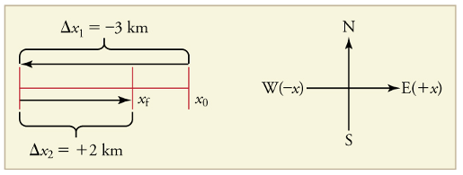
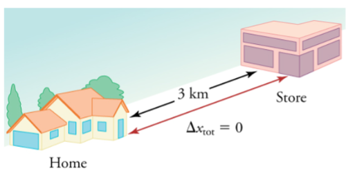
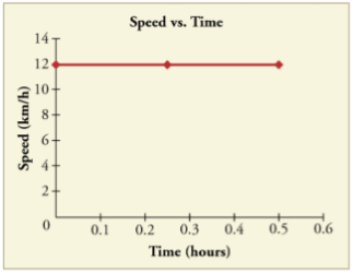
We have noted that distance traveled can be greater than displacement. So average speed can be greater than average velocity, which is displacement divided by time. For example, if you drive to a store and return home in half an hour, and your car’s odometer shows the total distance traveled was 6 km, then your average speed was 12 km/h. Your average velocity, however, was zero, because your displacement for the round trip is zero. (Displacement is change in position and, thus, is zero for a round trip.) Thus, average speed is not simply the magnitude of average velocity.
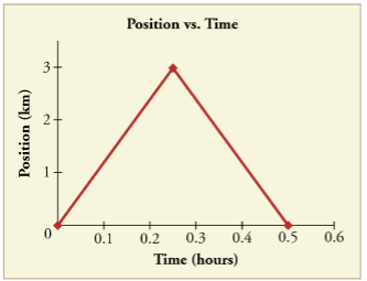
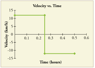
Another way of visualizing the motion of an object is to use a graph. A plot of position or of velocity as a function of time can be extremely useful. For example, for this trip to the store, the position, velocity, and speed-vs.-time graphs are displayed in Figures 6-8. (Note that these graphs depict a very simplified model of the trip. We are assuming that speed is constant during the trip, which is unrealistic given that we will probably stop at the store. But for simplicity’s sake, we will model it with no stops or changes in speed. We are also assuming that the route between the store and the house is a perfectly straight line.)
Acceleration:
In everyday conversation, to accelerate means to speed up. The accelerator in a car can in fact cause it to speed up. The greater the acceleration, the greater the change in velocity over a given time. The formal definition of acceleration is consistent with these notions, but more inclusive.
Average Acceleration is the rate at which velocity changes,

Where  is average acceleration, v is velocity, and t is time.
Because acceleration is velocity in m/s divided by time in s, the SI units for acceleration are  meters per second squared or meters per second per second, which means by how many meters per second the velocity changes every second.
Recall that velocity is a vector—it has both magnitude and direction. This means that a change in velocity can be a change in magnitude (or speed), but it can also be a change in direction. For example, if a car turns a corner at constant speed, it is accelerating because its direction is changing. The quicker you turn, the greater the acceleration. So, there is an acceleration when velocity changes either in magnitude (an increase or decrease in speed) or in direction, or both.
Keep in mind that although acceleration is in the direction of the change in velocity, it is not always in the direction of motion. When an object’s acceleration is in the same direction of its motion, the object will speed up. However, when an object’s acceleration is opposite to the direction of its motion, the object will slow down. Speeding up and slowing down should not be confused with a positive and negative acceleration.
Instantaneous Acceleration
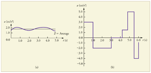
Instantaneous acceleration a, or the acceleration at a specific instant in time, is obtained by the same process as discussed for instantaneous velocity, that is by considering an infinitesimally small interval of time. How do we find instantaneous acceleration using only algebra? The answer is that we choose an average acceleration that is representative of the motion. Figure 9 shows graphs of instantaneous acceleration versus time for two quite different motions. In (a) the acceleration varies slightly and the average over the entire interval is nearly the same as the instantaneous acceleration at any time. In this case, we should treat this motion as if it had a constant acceleration equal to the average (in this case about  . In (b) the acceleration varies drastically over time. In such situations it is best to consider smaller time intervals and choose an average acceleration for each. For example, we could consider motion over the time intervals from 0 to 1.0 s and from 1.0 to 3.0 s as separate motions with accelerations of
  , respectively.
Check Your Understanding: The Motion of an Object in the Graphic Form through the Time-Space Diagram
Interpreting Motion Graphs
The Moving Man
Please complete this simulation.
Check Your Understanding: Interpreting Motion Graphs
Motion Diagram
Comparing Motion Diagrams (Simulation)
Please complete this simulation.
Use Kinematic Equations to Solve for Displacement, Time, Velocity and Acceleration of an Object
In this section, you will learn how to use kinematic equations to solve for displacement, time, velocity and acceleration of an object by reading each description. Also, short problems to check your understanding are included.
Motion Equations for Constant Acceleration in One Dimension
We might know that the greater the acceleration of, say, a car moving away from a stop sign, the greater the displacement in a given time. But we have not developed a specific equation that relates acceleration and displacement. In this section, we develop some convenient equations for kinematic relationships.
Notation: t, x, v, a
First, let us make some simplifications in notation. Taking the initial time to be zero, as if time is measured with a stopwatch, is a great simplification. Since elapsed time is  the final time on the stopwatch. When initial time is taken to be zero, we use the subscript 0 to denote initial values of position and velocity. That is, is the initial position and
  , is the initial velocity. We put no subscripts on the final values. The is, t is the final time, x is the final position, and v is final velocity. This gives a simpler expression for elapsed time – now,
  . It also simplifies the expression for displacement, which is now
  . Also, it simplifies the expression for change in velocity, which is now
  . To summarize, using the simplified notation, with the initial time taken to be zero,
Where the subscript 0 denotes an initial value and the absence of a subscript denotes a final value in whatever motion is under consideration.
We now make the important assumption that acceleration is constant. This assumption allows us to avoid using calculus to find instantaneous acceleration. Since acceleration is constant, the average and instantaneous accelerations are equal. That is,

So, we use the symbol a for acceleration at all times. Assuming acceleration to be constant does not seriously limit the situations we can study nor degrade the accuracy of our treatment. For one thing, acceleration is constant in a considerable number of situations. Furthermore, in many other situations we can accurately describe motion by assuming a constant acceleration equal to the average acceleration for that motion. Finally, in motions where acceleration changes drastically, such as a car accelerating to top speed and then braking to a stop, the motion can be considered in separate parts, each of which has its own constant acceleration.
Solving for Displacement () and the Final Position (x) from Average Velocity when Acceleration (a) is Constant.
To get our first two new equations, we start with the definition of average velocity:

Substituting the simplified notation for  yields

Solving for x yields

Where the average velocity is, with constant a

The equation reflects the fact that, when acceleration is constant, v is just the simple average of the initial and final velocities. For example, if you steadily increase your velocity (that is, with constant acceleration) from 30 to 60 km/h, then your average velocity during this steady increase is 45 km/h. Using the equation , we see that  .
.
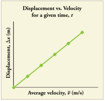
The equation gives insight into the relationship between displacement, average velocity, and time. It shows, for example, that displacement is a linear function of average velocity. (By linear function, we mean that displacement depends on rather than on raised to some other power, such as  . When graphed, linear functions look like straight lines with a constant slope.) On a car trip, for example, we will get twice as far in a given time if we average 90 km/h than if we average 45 km/h.
Solving for Final Velocity:
We can derive another useful equation by manipulating the definition of acceleration.

Substituting the simplified notation for  gives us (constant a)

Solving for v yields (constant a)

In addition to being useful in problem solving, the equation gives us insight into the relationships among velocity, acceleration, and time. From it we can see, for example that
- Final velocity depends on how large the acceleration is and how long it lasts
- If the acceleration is zero, then the final velocity equals the initial velocity
 , as expected (i.e., velocity is constant)
 - If a is negative, then the final velocity is less than the initial velocity.
Solving for Final Position when Velocity is Not Constant 
We can combine the equations above to find a third equation that allows us to calculate the final position of an object experiencing constant acceleration. We start with
Adding to each side of this equation and dividing by 2 gives

Since  for constant acceleration, then

Now we substitute this expression for into the equation for displacement, , yielding (constant a)

What else can we learn by examining the equation ? We see that:
- Displacement depends on the square of the elapsed time when acceleration is not zero.
- If acceleration is zero, then the initial velocity equals average velocity

Solving for Final Velocity when Velocity is not Constant 
A fourth useful equation can be obtained from another algebraic manipulation of previous equations.
If we solve  , we get

Substituting this and into , we get (constant a)

An examination of the equation can produce further insights into the general relationships among physical quantities:
- The final velocity depends on how large the acceleration is and the distance over which it acts
- For a fixed deceleration, a car that is going twice as fast does not simply stop in twice the distance – it takes much further to stop. (This is why we have reduced speed zones near schools).
Summary of Kinematic Equations (Constant a)
What are the Kinematic Formulas?
Please read “What Are Kinematic Formulas?”
Choosing Kinematic Equations
Free-body Diagrams
In this section, you will learn about free-body diagrams and how to make a free-body diagram by reading each description. Also, short problems to check your understanding are included.
Introduction to Forces and Free-body Diagrams
| Term | Meaning |
|---|---|
| Force | A push or pull on an object, usually has symbol F. Has SI units of Newtons  |
| Contact force | A force that requires contact between objects. Examples are tension, normal force, and friction. |
| Long range force | A force that does not need contact between objects to exist. |
| Free body diagram | A diagram showing the forces acting on the object. The object is represented by a dot with forces drawn as arrows pointing away from the dot. Sometimes called force diagrams. |
| Force (symbol) | Force type | Description |
|---|---|---|
Weight ( or W) or W) |
Long range | Force from gravity acting on an object with mass. Sometime called force of gravity. Pulls towards the Earth (down) always. |
Tension ( or T) or T) |
Contact | Force of something pulling on an object. Can be caused by a string, rope, chain, cord, cable, or wire. Pulls along the direction of the rope on the object. |
Normal force ( or N) or N) |
Contact | Force between two objects when they touch. Pushes perpendicularly to the object’s surface. |
Friction ( or f) or f) |
Contact | Force resisting sliding between surfaces. Pushes parallel to the contact surface and in the opposite direction of sliding. |
How to make a free body diagram:
-
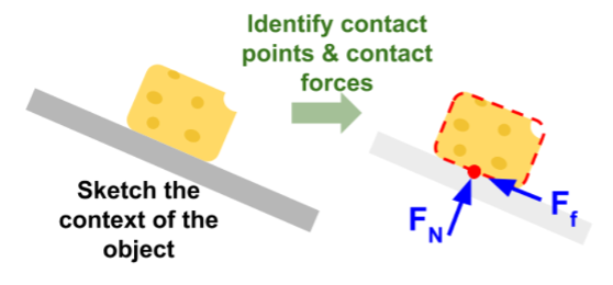
- Start by identifying the contact forces. Let us look for what the object is touching by outlining the object (see Figure 11). Draw a dot where something touches the outline; where there is a dot, there must be at least one contact force. Draw the force vectors at the contact points to represent how they push or pull on the object (including correct direction).
-
- After we have identified the contact forces, draw a dot to represent the object we are interested in (see Figure 12 in example). We only want to find the forces acting on our object and not forces the object exerts on other objects.
- Draw a coordinate system and label the positive directions. If the object is on an incline, then align the axes with the incline.
- Draw the contact forces on the dot with an arrow pointing away from the dot. Make sure the arrow lengths are relatively proportional to each other. Label all forces.
- Draw and label our long-range forces. This will usually be weight unless there is electric charge or magnetism involved.
- Draw and label your acceleration vector off to the side of the dot – not touching the dot. If there is no acceleration, then write
 .
.
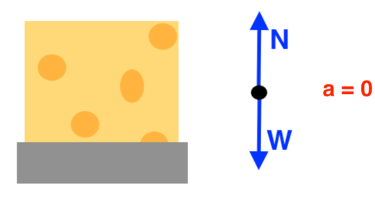
Here is an example of a free body diagram for a block of cheese resting on a table (See Figure 12). Gravity pulls down on the cheese’s mass with weight (W) and the table pushes up on the cheese with a normal force (N). Since there are no ropes and the cheese is not trying to slide, there is no tension or friction.
Common mistakes and misconceptions
-
- Sometimes people draw the forces of the object acting on other things. We only want to draw the forces pushing or pulling on our object. Only focus on what is happening to the object of interest.
- Sometimes people forget the directions of the different types of forces. Weight is always down, friction is always parallel to the contact surface, normal force is always perpendicular to the contact surface, and tension only pulls.
Check Your Understanding: Forces and Free-body Diagrams
Estimate the Friction Force and Normal Reaction on a Static Object
In this section, you will learn how estimate the friction force and normal reaction on a static object and learn about kinetic and static friction forces by reading each description along with watching the videos. Also, short problems to check your understanding are included.
Normal Force
If the force supporting a load is perpendicular to the surface of contact between the load and its support, this force is defined to be a normal force and is given the symbol N (different from newton). The word normal means perpendicular to a surface.
Friction
Friction is a force that opposes relative motion between systems in contact. One of the simpler characteristics of friction is that it is parallel to the contact surface between systems and always in a direction that opposes motion or attempted motion of the systems relative to each other. If two systems are in contact and moving relative to one another, then the friction between them is called kinetic friction. For example, friction slows a hockey puck sliding on ice. But when objects are stationary, static friction can act between them; the static friction is usually greater than the kinetic friction between the objects.
As seen in Table 1 below, the coefficients of kinetic friction are less than their static counterparts. The equations explained below include the dependence of friction on materials and the normal force.
| System |  Static Function Static Function |
 Kinetic Function Kinetic Function |
|---|---|---|
| Rubber on dry concrete | 1.0 | 0.7 |
| Rubber on wet concrete | 0.7 | 0.5 |
| Wood on wood | 0.5 | 0.3 |
| Waxed wood on wet snow | 0.14 | 0.1 |
| Metal on wood | 0.5 | 0.3 |
| Steel on steel (dry) | 0.6 | 0.3 |
| Steel on steel (oiled) | 0.05 | 0.03 |
| Teflon on steel | 0.04 | 0.04 |
| Bone lubricated by synovial fluid | 0.016 | 0.015 |
| Shoes on wood | 0.9 | 0.7 |
| Shoes on ice | 0.1 | 0.05 |
| Ice on ice | 0.1 | 0.03 |
| Steel on ice | 0.04 | 0.02 |
Kinetic and Static Friction Forces
Static Friction Equation
Where there is no motion between the objects, the magnitude of static friction is  is the coefficient of static friction and N is the magnitude of the normal force.
The symbol  means less than or equal to, implying that static friction can have a minimum and a maximum value of
  . Static friction is a responsive force that increases to be equal and opposite to whatever force is exerted, up to its maximum limit. Once the applied force exceeds
  , the object will move. Thus
  .
.
Kinetic Friction Equation
Once an object is moving, the magnitude of kinetic friction  is given by
  is the coefficient of kinetic friction.
Check Your Understanding: Friction
Static and Kinetic Friction Example
Check Your Understanding: Static and Kinetic Friction
Forces and Newton’s Laws
In this section, you will learn about Newton’s three laws of motion along with laws of gravitation by reading each description along with watching the videos. Also, short problems to check your understanding are included.
Newton’s 3 Laws of Motion
Newton’s First Law of Motion
There exists an inertial frame of reference such that a body at rest remains at rest, or, if in motion, remains in motion at a constant velocity unless acted on by a net external force.
The first law of motion postulates the existence of at least one frame of reference which we call an inertial reference frame, relative to which the motion of an object not subject to forces is a straight line at a constant speed. An inertial reference frame is any reference frame that is not itself accelerating. A car traveling at constant velocity is an inertial reference frame. A car slowing down for a stoplight, or speeding up after the light turns green, will be accelerating and is not an inertial reference frame. Finally, when the car goes around a turn, which is due to an acceleration changing the direction of the velocity vector, it is not an inertial reference frame. Note that Newton’s laws of motion are only valid for inertial reference frames.
Rather than contradicting our experience, Newton’s first law of motion states that there must be a cause (which is a net external force) for there to be any change in velocity (either a change in magnitude or direction) in an inertial reference frame. An object sliding across a table or floor slows down due to the net force of friction acting on the object.
The idea of cause and effect is crucial in accurately describing what happens in various situations. For example, consider what happens to an object sliding along a rough horizontal surface. The object quickly grinds to a halt. If we spray the surface with talcum powder to make the surface smoother, the object slides farther. If we make the surface even smoother by rubbing lubricating oil on it, the object slides farther yet. Extrapolating to a frictionless surface, we can imagine the object sliding in a straight line indefinitely. Friction is thus the cause of the slowing (consistent with Newton’s first law). The object would not slow down at all if friction were completely eliminated. Consider an air hockey table. When the air is turned off, the puck slides only a short distance before friction slows it to a stop. However, when the air is turned on, it creates a nearly frictionless surface, and the puck glides long distances without slowing down. Additionally, if we know enough about the friction, we can accurately predict how quickly the object will slow down. Friction is an external force.
Mass: The property of a body to remain at rest or to remain in motion with constant velocity is called inertia. Newton’s first law is often called the law of inertia. As we know from experience, some objects have more inertia than others. It is obviously more difficult to change the motion of a large boulder than that of a basketball, for example. The inertia of an object is measured by its mass.
An object with a small mass will exhibit less inertia and be more affected by other objects. An object with a large mass will exhibit greater inertia and be less affected by other objects. This inertial mass of an object is a measure of how difficult it is to alter the uniform motion of the object by an external force.
Roughly speaking, mass is a measure of the amount of “stuff” (or matter) in something. The quantity or amount of matter in an object is determined by the numbers of atoms and molecules of several types it contains. Unlike weight, mass does not vary with location. The mass of an object is the same on Earth, in orbit, or on the surface of the Moon. In practice, it is exceedingly difficult to count and identify all of the atoms and molecules in an object, so masses are not often determined in this manner. Operationally, the masses of objects are determined by comparison with the standard kilogram.
Check Your Understanding: Newton’s First Law of Motion
Newton’s Second Law of Motion
Newton’s second law of motion is closely related to Newton’s first law of motion. It mathematically states the cause-and-effect relationship between force and changes in motion. Newton’s second law of motion is more quantitative and is used extensively to calculate what happens in situations involving a force. Before we can write down Newton’s second law as a simple equation giving the exact relationship of force, mass, and acceleration, we need to sharpen some ideas that have already been mentioned.
First, what do we mean by a change in motion? The answer is that a change in motion is equivalent to a change in velocity. A change in velocity means, by definition, that there is an acceleration. Newton’s first law says that a net external force causes a change in motion; thus, we see that a net external force causes acceleration.
Another question immediately arises. What do we mean by an external force? An intuitive notion of external is correct—an external force acts from outside the system of interest. An internal force acts between elements of the system. Only external forces affect the motion of a system, according to Newton’s first law.
To obtain an equation for Newton’s Second Law, we first write the relationship of acceleration and net external force as the proportionality

Where the symbol  means “proportional to,” and
  is the net external force. This proportionality states acceleration is directly proportional to the net external force. Now, it also seems reasonable that acceleration should be inversely proportional to the mass of the system. In other words, the larger the mass (the inertia), the smaller the acceleration produced by a given force. This proportionality is written as
  , where m is the mass of the system. Combining the two proportionalities just given yield’s Newton’s Second Law of Motion.
Newton’s Second Law of Motion: The acceleration of a system is directly proportional to and in the same direction as the net external force acting on the system, and inversely proportional to its mass. In equation form, Newton’s Second Law of Motion is:

Often written as:

Units of Force: is used to define the units of force in terms of the three basic units for mass, length, and time. The SI unit of force is called the newton (abbreviated N) and is the force needed to accelerate a 1-kg system at the rate of  . That is, since
  .
.
Weight and the Gravitational Force: When an object is dropped, it accelerates toward the center of Earth. Newton’s second law states that a net force on an object is responsible for its acceleration. If air resistance is negligible, the net force on a falling object is the gravitational force, commonly called its weight w.
Since the object experiences only the downward force of gravity,  . We know that the acceleration of an object due to gravity is
  . Substituting these into Newton’s Second Law gives
  . Since
  on Earth, the weight of a 1.0 kg object on Earth is 9.81N, as we see:
  .
.
When the net external force on an object is its weight, we say that it is in free-fall. That is, the only force acting on the object is the force of gravity. In the real world, when objects fall downward toward Earth, they are never truly in free-fall because there is always some upward force from the air acting on the object.
Common misconceptions: Mass vs. Weight: It is important to be aware that weight and mass are very different physical quantities, although they are closely related. Mass is the quantity of matter (how much “stuff”) and does not vary in classical physics, whereas weight is the gravitational force and does vary depending on gravity. It is tempting to equate the two, since most of our examples take place on Earth, where the weight of an object only varies a little with the location of the object.
Check Your Understanding: Newton’s Second Law of Motion
Newton’s Third Law of Motion
Whenever one body exerts a force on a second body, the first body experiences a force that is equal in magnitude and opposite in direction to the force that it exerts.
This law represents a certain symmetry in nature: Forces always occur in pairs, and one body cannot exert a force on another without experiencing a force itself. We sometimes refer to this law loosely as “action-reaction,” where the force exerted is the action and the force experienced as a consequence is the reaction. Newton’s third law has practical uses in analyzing the origin of forces and understanding which forces are external to a system. You might think that two equal and opposite forces would cancel, but they do not because they act on different systems.
Other examples of Newton’s third law are easy to find. As a professor paces in front of a whiteboard, she exerts a force backward on the floor. The floor exerts a reaction force forward on the professor that causes her to accelerate forward. Similarly, a car accelerates because the ground pushes forward on the drive wheels in reaction to the drive wheels pushing backward on the ground. You can see evidence of the wheels pushing backward when tires spin on a gravel road and throw rocks backward.
In another example, rockets move forward by expelling gas backward at high velocity. This means the rocket exerts a large backward force on the gas in the rocket combustion chamber, and the gas therefore exerts a large reaction force forward on the rocket. This reaction force is called thrust. It is a common misconception that rockets propel themselves by pushing on the ground or on the air behind them. They actually work better in a vacuum, where they can more readily expel the exhaust gases. Helicopters similarly create lift by pushing air down, thereby experiencing an upward reaction force. Birds and airplanes also fly by exerting force on air in a direction opposite to that of whatever force they need.
Check Your Understanding: Newton’s Third Law of Motion
Gravity Force Lab
Laws of Gravitation
Newton’s Universal Law of Gravitation
The gravitational force is relatively simple. It is always attractive, and it depends only on the masses involved and the distance between them. Stated in modern language, Newton's universal law of gravitation states that every particle in the universe attracts every other particle with a force along a line joining them. The force is directly proportional to the product of their masses and inversely proportional to the square of the distance between them.
Misconception alert: The magnitude of the force on each object (one has larger mass than the other) is the same, consistent with Newton’s Third Law.
For two bodies having masses m and M with a distance r between their centers of mass, the equation for Newton’s Universal Law of Gravitation is

Where F is the magnitude of the gravitation force and G is a proportionality factor called the gravitational constant. G is a universal gravitational constant—that is, it is thought to be the same everywhere in the universe. It has been measured experimentally to be in SI units,

Introduction to Spatial Interaction Modelling
Check Your Understanding: Spatial Interaction Modelling
Describe the Motion of an Object Along a Circular Path
In this section, you will learn about the motion of an object along a circular path by reading each description along with watching the videos. Also, short problems to check your understanding are included.
Angular Rotation
Angle Units
Angular Position and Displacement
Angular Velocity and Acceleration
Uniform Circular Motion
Rotation Angle and Angular Velocity
We begin the study of uniform circular motion by defining two angular quantities needed to describe rotational motion.
Rotation Angle
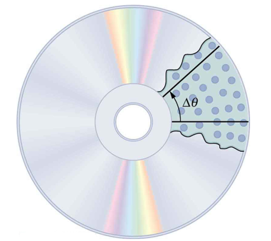
When objects rotate about some axis – for example, when the CD in Figure 13 below rotates about its center – each point in the object follows a circular arc. Consider a line from the center of the CD to its edge. Each pit used to record sound along this line moves through the same angle in the same amount of time. The rotation angle is the amount of rotation and is analogous to linear distance. We define the rotation angle  to be the ratio of the arc length to the radius of curvature:


The arc length  is the distance traveled along a circular path as shown in Figure 14 below. Note that r is the radius of curvature of the circular path.
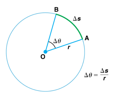 . The arc length is described on the circumference.
We know that for one complete revolution, the arc length is the circumference of a circle of radius r. The circumference of a circle is  . Thus, for one complete revolution the rotation angle is

This result is the basis for defining the units used to measure rotation angles, to be radians (rad), defined so that

A comparison of some useful angles expressed in both degrees and radians is shown in Table 2 below.
| Degree Measures | Radian Measure |
|---|---|
| 30° |  |
| 60° |  |
| 90° |  |
| 120° |  |
| 135° |  |
| 180° |  |
Angular Velocity
How fast is an object rotating? We define angular velocity  as the rate of change of an angle. In symbols, this is

Where an angular rotation takes place in a time . The greater the rotation angle in a given amount of time, the greater the angular velocity. The units for angular velocity are radians per second (rad/s).
Angular velocity  is analogous to linear velocity v. To get the precise relationship between angular and linear velocity, we again consider a pit on the rotating CD. This pit moves an arc length in a time , and so it has a linear velocity

From we see that  . Substituting this into the expression for v gives

We write this relationship in two different ways and gain two different insights:

The first relationship in states that the linear velocity v is proportional to the distance from the center of rotation, thus, it is the largest for a point on the rim (larges r), as you might expect. We can also call this linear speed v of a point on the rim the tangential speed. The second relationship in can be illustrated by considering the tire of a moving car. Note that the speed of a point on the rim of the tire is the same as the speed v of the car. See Figure 15 below. So, the faster the car moves, the faster the tire spins – large v means a large , because  . Similarly, a larger-radius tire rotating at the same angular velocity () will produce a greater linear speed (v) for the car.
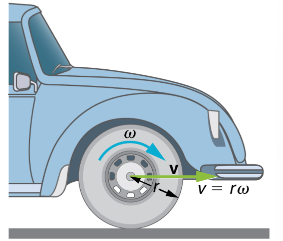 . The speed of the tread of the tire relative to the axle is v, the same as if the car were jacked up. Thus, the car moves forward at linear velocity , where r is the tire radius. A larger angular velocity for the tire means a greater velocity for the car.
Check Your Understanding: Angular Rotation
Circular Motion and Centripetal Acceleration
Centripetal Force and Acceleration Intuition
Visual Understanding of Centripetal Acceleration Formula
Centripetal Acceleration
We know from kinematics that acceleration is a change in velocity, either in its magnitude or in its direction, or both. In uniform circular motion, the direction of the velocity changes constantly, so there is always an associated acceleration, even though the magnitude of the velocity might be constant. You experience this acceleration yourself when you turn a corner in your car. (If you hold the wheel steady during a turn and move at constant speed, you are in uniform circular motion.) What you notice is a sideways acceleration because you and the car are changing direction. The sharper the curve and the greater your speed, the more noticeable this acceleration will become. In this section we examine the direction and magnitude of that acceleration.
Figure 16 below shows an object moving in a circular path at constant speed. The direction of the instantaneous velocity is shown at two points along the path. Acceleration is in the direction of the change in velocity, which points directly toward the center of rotation (the center of the circular path). This pointing is shown with the vector diagram in the figure. We call the acceleration of an object moving in uniform circular motion (resulting from a net external force) the centripetal acceleration ( ); centripetal means “toward the center” or “center seeking.”
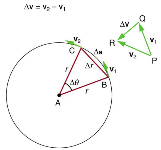
 is seen to point directly toward the center of curvature. (See small inset). Because
  , the acceleration is also toward the center; is called centripetal acceleration. (Because is exceedingly small, the arc length
  is equal to the chord length
  for small time differences).
The direction of centripetal acceleration is toward the center of curvature, but what is its magnitude? Note that the triangle formed by the velocity vectors and the one formed by the radii r and are similar. Both the triangles ABC and PQR are isosceles triangles (two equal sides). The two equal sides of the velocity vector triangle are the speeds  . Using the properties of two similar triangles, we obtain

Acceleration is  , and so we first solve this expression for :

Then we divide this by , yielding

Finally, noting that  , and that
  , the linear or tangential speed, we see that the magnitude of the centripetal acceleration is

Which is the acceleration of an object in a circle of radius r at a speed v. So, centripetal acceleration is greater at high speeds and in sharp curves (smaller radius), as you have noticed when driving a car. But it is a bit surprising that is proportional to speed squared, implying, for example, that it is four times as hard to take a curve at 100 km/h than at 50 km/h. A sharp corner has a small radius, so that is greater for tighter turns, as you have probably noticed.
It is also useful to express in terms of angular velocity. Substituting into the above expression, we find  . We can express the magnitude of centripetal acceleration using either of the two equations:

Recall that the direction of is toward the center. You may use whichever expression is more convenient.
Check Your Understanding: Circular Motion and Centripetal Acceleration
Centripetal Forces
Centripetal Force Problem Solving
Centripetal Force
Any force or combination of forces can cause a centripetal or radial acceleration. Just a few examples are the tension in the rope on a tether ball, the force of Earth’s gravity on the Moon, friction between roller skates and a rink floor, a banked roadway’s force on a car, and forces on the tube of a spinning centrifuge.
Any net force causing circular motion is called a centripetal force. The direction of a centripetal force is toward the center of curvature, the same as the direction of centripetal acceleration. According to Newton’s Second Law of Motion, the net force is mass times acceleration:  . For uniform circular motion, the acceleration is the centripetal acceleration –
  . Thus, the magnitude of centripetal force
  is
is

By using the expressions for centripetal acceleration  ;
;  , we get two expressions for the centripetal force in terms of mass, velocity, angular velocity, and radius of curvature:

You may use whichever expression for centripetal force is more convenient. Centripetal force is always perpendicular to the path and pointing to the center of curvature, because is perpendicular to the velocity and pointing to the center of curvature.
Note that if you solve the first expression for r, you get

This implies that for a given mass and velocity, a large centripetal force causes a small radius of curvature – that is, a tight curve.
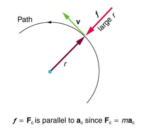 , the smaller the radius of curvature r and the sharper the curve.
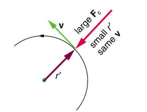 , the smaller the radius of curvature r and the sharper the curve. This curve has the same v, but a larger produces a smaller r’.
Example 1
- What coefficient of friction do car tires need on a flat curve?
(a) Calculate the centripetal force exerted on a 900 kg car that negotiates a 500 m radius curve as .
.
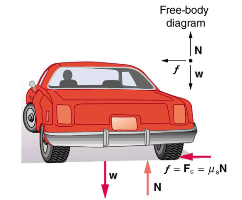
(b) Assuming an unbanked curve, find the minimum statis coefficient of friction, between the tires and the road, static friction being the reason that keeps the car from slipping (See Figure 19 below).
Answer: (a) 
(b) Figure 19 shows the forces acting on the car on an unbanked (level ground) curve. Friction is to the left, keeping the car from slipping, and because it is the only horizontal force acting on the car, the friction is the centripetal force in this case. We know that the maximum static friction (at which the tires roll but do not slip) is  is the static coefficient of friction and N is the normal force. The normal force equals the car’s weight on level ground, so that
  . Thus the centripetal force in this situation is

Now we have a relationship between centripetal force and the coefficient of friction. Using the first expression for from the equation


We solve this for  , noting that mass cancels, and obtain

Substituting the knowns,

Let us now consider banked curves, where the slope of the road helps you negotiate the curve. See Figure 20 below. The greater the angle  , the faster you can take the curve. Racetracks for bikes as well as cars, for example, often have steeply banked curves. In an “ideally banked curve,” the angle is such that you can negotiate the curve at a certain speed without the aid of friction between the tires and the road. We will derive an expression for for an ideally banked curve and consider an example related to it.
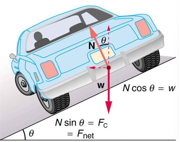
For ideal banking, the net external force equals the horizontal centripetal force in the absence of friction. The components of the normal force N in the horizontal and vertical directions must equal the centripetal force and the weight of the car, respectively. In cases in which forces are not parallel, it is most convenient to consider components along perpendicular axes – in this case, the vertical and horizontal directions.
Figure 20 above shows a free-body diagram for a car on a frictionless banked curve. If the angle is ideal for the speed and radius, then the net external force will equal the necessary centripetal force. The only two external forces acting on the car are its weight w and the normal force of the road N. (A frictionless surface can only exert a force perpendicular to the surface – that is, a normal force). These two forces must add to give a net external force that is horizontal toward the center of curvature and has magnitude  . Because this is the crucial force and it is horizontal, we use a coordinate system with vertical and horizontal axes. Only the normal force has a horizontal component, and so this must equal the centripetal force – that is,

Because the car does not leave the surface of the road, the net vertical force must be zero, meaning that the vertical components of the two external forces must be equal in magnitude and opposite in direction. From the figure, we see that the vertical component of the normal force is N cos , and the only other vertical force is the car’s weight. These must be equal in magnitude; thus,

Now we can combine the last two equations to eliminate N and get an expression for , as desired. Solving the second equation for  , and substituting this into the first yields

m g \tan (\theta)=\frac{m v^2}{r}

Taking the inverse tangent gives

This expression can be understood by considering how depends on v and r. A large will be obtained for a large v and a small r. That is, roads must be steeps banked for high speeds and sharp curves. Friction helps, because it allows you to take the curve at greater or lower speed than if the curve is frictionless. Note that does not depend on the mass of the vehicle
Example 2
- What is the ideal speed to take a steeply banked tight curve? Curves on some test tracks and racecourses, such as the Daytona International Speedway in Florida, are very steeply banked. This banking, with the aid of tire friction and very stable car configurations, allows the curves to be taken at very high speed. To illustrate, calculate the speed at which a 100 m radius curve banked at
 should be driven if the road is frictionless.
Answer: 
Noting that  , we obtain
![v=\left[(100 m)\left(\frac{9.80 m}{s^2}\right)(2.14)\right]^{\frac{1}{2}}=45.8 \mathrm{~m} / \mathrm{s}](https://uta.pressbooks.pub/app/uploads/quicklatex/quicklatex.com-d4447badf03d9e985475c34e528f642b_l3.png "Rendered by QuickLaTeX.com")
Frames of Reference
Fictitious Forces
Fictitious Forces and Non-Inertial Frames: The Coriolis Force
What do taking off in a jet airplane, turning a corner in a car, riding a merry-go-round, and the circular motion of a tropical cyclone have in common? Each exhibits fictitious forces—unreal forces that arise from motion and may seem real, because the observer’s frame of reference is accelerating or rotating.
When taking off in a jet, most people would agree it feels as if you are being pushed back into the seat as the airplane accelerates down the runway. Yet a physicist would say that you tend to remain stationary while the seat pushes forward on you, and there is no real force backward on you. An even more common experience occurs when you make a tight curve in your car—say, to the right. You feel as if you are thrown (that is, forced) toward the left relative to the car. Again, a physicist would say that you are going in a straight line, but the car moves to the right, and there is no real force on you to the left. Recall Newton’s first law.
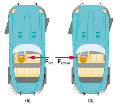
We can reconcile these points of view by examining the frames of reference used. Let us concentrate on people in a car. Passengers instinctively use the car as a frame of reference, while a physicist uses Earth. The physicist chooses Earth because it is very nearly an inertial frame of reference—one in which all forces are real (that is, in which all forces have an identifiable physical origin). The car is a non-inertial frame of reference because it is accelerated to the side. The force to the left sensed by car passengers is a fictitious force having no physical origin. There is nothing real pushing them left—the car, as well as the driver, is actually accelerating to the right.
Let us now take a mental ride on a merry-go-round—specifically, a rapidly rotating playground merry-go-round. You take the merry-go-round to be your frame of reference because you rotate together. In that non-inertial frame, you feel a fictitious force, named centrifugal force (not to be confused with centripetal force), trying to throw you off. You must hang on tightly to counteract the centrifugal force. In Earth’s frame of reference, there is no force trying to throw you off. Rather you must hang on to make yourself go in a circle because otherwise you would go in a straight line, right off the merry-go-round.
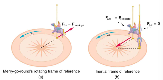
 and heads in a straight line). A real force,
  , is needed to cause a circular path.
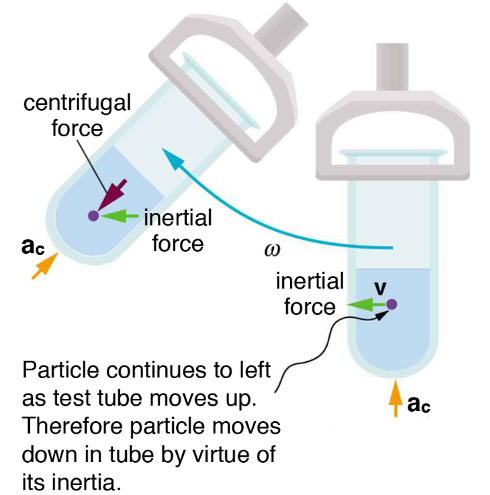
This inertial effect, carrying you away from the center of rotation if there is no centripetal force to cause circular motion, is put to good use in centrifuges (See Figure 23). A centrifuge spins a sample very rapidly. Viewed from the rotating frame of reference, the fictitious centrifugal force throws particles outward, hastening their sedimentation. The greater the angular velocity, the greater the centrifugal force. But what really happens is that the inertia of the particles carries them along a line tangent to the circle while the test tube is forced in a circular path by a centripetal force.
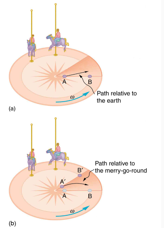
Let us now consider what happens if something moves in a frame of reference that rotates. For example, what if you slide a ball directly away from the center of the merry-go-round, as shown in Figure 24 below? The ball follows a straight path relative to Earth (assuming negligible friction) and a path curved to the right on the merry-go-round’s surface. A person standing next to the merry-go-round sees the ball moving straight and the merry-go-round rotating underneath it. In the merry-go-round’s frame of reference, we explain the apparent curve to the right by using a fictitious force, called the Coriolis force, which causes the ball to curve to the right. The fictitious Coriolis force can be used by anyone in that frame of reference to explain why objects follow curved paths and allows us to apply Newton’s Laws in non-inertial frames of reference.
Relevance to Transportation Engineering Coursework
This section explains the relevance of trip distribution, superelevation, stopping sight distance, time and space headways to transportation engineering coursework.
Trip Distribution
In travel demand modeling, one of the major steps (typically Step 2 of the 4-step process) involves estimating the number of trips made from one designated traffic analysis zone (TAZ) to another. This step is termed the trip distribution step. There are multiple trip distribution computational techniques, or “models,” and the gravity model, derived from the physics gravity model (see the above section titled “Laws of Gravitation”), is one of the most useful models. In the physics gravity model, the greater the masses of two objects and the shorter the distance between them, the greater the gravitational pull. In the trip distribution step, the total number of trips produced at the origin zone and attracted at the destination zone are analogous to the object masses. Furthermore, just like the gravity model from Physics, the number of trips is also inversely proportional to an exponent of the distance between zones.
Superelevation
The above section titled “Circular Motion and Centripetal Acceleration” describes the basics of circular motion. This understanding and the discussion on the balancing of forces in Chapter 6 are critical to the cross-section design of the road segments with horizontal curves.
Stopping Sight Distance
The stopping sight distance, SSD, is the distance needed for a driver to perceive an unusual situation and stop to avoid crashing into an object or another road user. The SSD is estimated based on the time needed for the driver to detect and recognize the situation, also known as perception-reaction time (PRT), and the distance needed to brake to a complete stop, also known as the braking distance. These distances are estimated using the principles of kinematics for motion at constant speeds (see the above section titled ” 1.1 Describe the Motion of an Object in the Graphic Form through the Time-Space Diagram”), with accelerated motion (see sections “Motion Equations for Constant Acceleration in One Dimension” and “What are the Kinematic Formulas?”), and traveling along a grade (see the section titled “Forces and Newton’s Laws”).
Time and Space Headways
The time headway is the time difference between the front bumper of one vehicle and that of another traveling behind it, passing the same point on a roadway segment. Space headway is the physical distance between the front bumper of a vehicle and that of another behind it. The relationship between time and space headways is based on kinematic relationships discussed in the sections titled “Time, Velocity, Speed, and Acceleration” and ” Use Kinematic Equations to Solve for Displacement, Time, Velocity and Acceleration of an Object”. The time headway may be used to estimate the traffic flow rate at points of the roadway segments. It is defined as the number of vehicles passing a point on the road per unit of time (in the units of vehicles/hour). The space headway may be used to estimate the density of the traffic stream on a roadway segment. It is the number of vehicles observed per unit distance on a roadway stretch (vehicles/mile).
Key Takeaways
- The gravity model from physics described in the chapter provides the foundational understanding of the trip distribution modeling between traffic analysis zones (TAZs). The gravity model is based on the idea that the number of trips between two zones is related to the size of the zones (i.e., total trips produced/attracted at a zone based on characteristics such as population or employment) and the distance between them.
- To ensure safe travel, the SSD (Stopping Sight Distance) is estimated based on the design speed appropriate for the roadway segments. Principles of kinematics for motion discussed in this chapter are used to derive formulas for estimating SSD appropriate for the context.
- The idea of motion at constant speed also relates to the time and space headways between vehicles and is useful for estimating flow rate past a point and density on roadway segments.
Glossary: Key Terms
Acceleration[1] – the rate at which an object’s velocity changes over a period of time
Acceleration due to Gravity[1] – acceleration of an object as result of gravity
Accuracy[1] – the degree to which a measured value agrees with correct value for that measurement
Angular Velocity[1]– 𝜔, the rate of change of the angle with which an object moves on a circular path
Arc Length[1]– ∆𝑠, the distance traveled by an object along a circular path
Average Acceleration[1] – the change in velocity divided by the time over which it changes
Average Speed[1] – distance traveled divided by time during which motion occurs
Average Velocity[1] – displacement divided by the time over which displacement occurs
Banked Curve[1] – the curve in a road that is sloping in a manner that helps a vehicle negotiate the curve
Center of Mass[1] – the point where the entire mass of an object can be thought to be concentrated
Centrifugal Force[1] – a fictitious force that tends to throw an object off when the object is rotating in a non-inertial frame of reference
Centripetal Acceleration[1] – the acceleration of an object moving in a circle, directed toward the center
Centripetal Force[1] – any net force causing uniform circular motion
Classical Physics[1] – physics that was developed from the Renaissance to the end of the 19th century
Conversion Factor[1] – a ratio expressing how many of one unit are equal to another unit
Coriolis Force[1] – the fictitious force causing the apparent deflection of moving objects when viewed in a rotating frame of reference
Deceleration[1] – acceleration in the direction opposite to velocity; acceleration that results in a decrease in velocity
Displacement[1] – the change in position of an object
Distance[1] – the magnitude of displacement between two positions
Distance Traveled[1] – the total length of the path traveled between two positions
Elapsed Time[1] – the difference between the ending time and beginning time
English Units[1] – system of measurement used in the United States; includes units of measurement such as feet, gallons, and pounds
External Force[1] – a force acting on an object or system that originates outside of the object or system
Fictious Force[1] – a force having no physical origin
Force[1] – a push or pull on an object with a specific magnitude and direction; can be represented by vectors; can be expressed as a multiple of a standard force
Free-body Diagram[1] – a sketch showing all of the external forces acting on an object or system; the system is represented by a dot, and the forces are represented by vectors extending outward from the dot
Free-Fall[1] – a situation in which the only force acting on an object is the force due to gravity
Friction[1] – a force past each other of objects that are touching; examples include rough surfaces and air resistance
Gravitational Constant, G[1] – a proportionality factor used in the equation for Newton’s universal law of gravitation; it is a universal constant—that is, it is thought to be the same everywhere in the universe
Ideal Banking[1] – the sloping of a curve in a road, where the angle of the slope allows the vehicle to negotiate the curve at a certain speed without the aid of friction between the tires and the road; the net external force on the vehicle equals the horizontal centripetal force in the absence of friction
Ideal Speed[1] – the maximum safe speed at which a vehicle can turn on a curve without the aid of friction between the tire and the road
Inertia[1] – the tendency of an object to remain at rest or remain in motion
Inertial Frame of Reference[1] – a coordinate system that is not accelerating; all forces acting in an inertial frame of reference are real forces, as opposed to fictitious forces that are observed due to an accelerating frame of reference
Instantaneous Acceleration[1]– acceleration at a specific point in time
Instantaneous Speed[1] – magnitude of the instantaneous velocity
Instantaneous Velocity[1] – velocity at a specific instant, or the average velocity over an infinitesimal time interval
Kilogram[1] – the SI unit for mass, abbreviated (kg)
Kinematics[1] – the study of motion without considering its causes
Kinetic Friction[1] – a force that opposes the motion of two systems that are in contact and moving relative to one another
Law[1] – a description, using concise language or a mathematical formula, a generalized pattern in nature that is supported by scientific evidence and repeated experiments
Law of Inertia[1] – see Newton’s first law of motion
Magnitude of Kinetic Friction[1] – 𝑓𝑘=𝜇𝑘𝑁, where 𝜇𝑘 is the coefficient of kinetic friction
Magnitude of Static Friction[1] – 𝑓𝑠≤𝜇𝑠𝑁, where 𝜇𝑠 is the coefficient of static friction and 𝑁 is the magnitude of the normal force
Mass[1] – the quantity of matter in a substance; measured in kilograms
Meter[1] – the SI unit for length, abbreviated (m)
Metric System[1]– a system in which values can be calculated in factors of 10
Model[1]– simplified description that contains only those elements necessary to describe the physics of a physical situation
Net External Force[1] – the vector sum of all external forces acting on an object or system; causes a mass to accelerate
Newton’s First Law of Motion[1]– in an inertial frame of reference, a body at rest remains at rest, or, if in motion, remains in motion at a constant velocity unless acted on by a net external force; also known as the law of inertia
Newton’s Second Law of Motion[1] – the net external force 𝐹𝑛𝑒𝑡 on an object with mass 𝑚 is proportional to and in the same direction as the acceleration of the object, 𝑎, and inversely proportional to the mass; defined mathematically as
Newton’s Third Law of Motion[1] – whenever one body exerts a force on a second body, the first body experiences a force that is equal in magnitude and opposite in direction to the force that the first body exerts
Newton’s Universal Law of Gravitation[1] – every particle in the universe attracts every other particle with a force along a line joining them; the force is directly proportional to the product of their masses and inversely proportional to the square of the distance between them
Non-Inertial Frame of Reference[1]– an accelerated frame of reference
Normal Force[1] – the force that a surface applies to an object to support the weight of the object; acts perpendicular to the surface on which the object rests
Physical Quantity[1] – a characteristic or property of an object that can be measured or calculated from other measurements
Physics[1] – the science concerned with describing the interactions of energy, matter, space, and time; it is especially interested in what fundamental mechanisms underlie every phenomenon
Pit[1] – a tiny indentation on the spiral track moulded into the top of the polycarbonate layer of CD
Position[1] – the location of an object at a particular time
Radians[1] – a unit of angle measurement
Radius of Curvature[1]– radius of a circular path
Rotation Angle[1] – the ratio of arc length to the radius of curvature on a circular path:
Scalar[1] – a quantity that is described by magnitude, but not direction
Second[1]– the SI unit for time, abbreviated (s)
SI Units[1]– the international system of units that scientists in most countries have agreed to use; includes units such as meters, liters, and grams
Significant Figures[1] – express the precision of a measuring tool used to measure a value
Slope[1] – the difference in y-value (the rise) divided by the difference in x-value (the run) of two points on a straight line
Static Friction[1] – a force that opposes the motion of two systems that are in contact and are not moving relative to one another
System[1]– defined by the boundaries of an object or collection of objects being observed; all forces originating from outside of the system are considered external forces
Tension[1] – the pulling force that acts along a medium, especially a stretched flexible connector, such as a rope or cable; when a rope supports the weight of an object, the force on the object due to the rope is called a tension force
Thrust[1]– a reaction force that pushes a body forward in response to a backward force; rockets, airplanes, and cars are pushed forward by a thrust reaction force
Time[1]– change, or the interval over which change occurs
Ultracentrifuge[1] – a centrifuge optimized for spinning a rotor at very high speeds
Uniform Circular Motion[1] – the motion of an object in a circular path at constant speed
Units[1] – a standard used for expressing and comparing measurements
Vector[1] – a quantity that is described by both magnitude and direction
Weight[1] – the force 𝑤 due to gravity acting on an object of mass 𝑚; defined mathematically as: 𝑤=𝑚𝑔, where 𝑔 is the magnitude and direction of the acceleration due to gravity
Y-Intercept[1] – the y-value when 𝑥=0, or when the graph crosses the y-axis
[1] “College Physics for AP® Courses” by Greg Wolfe, Erika Gasper, John Stoke, Julie Kretchman, David Anderson, Nathan Czuba, Sudhi Oberoi, Liza Pujji, Irina Lyublinskaya, Douglas Ingram. Access for free at https://openstax.org/books/college-physics-ap-courses/pages/1-connection-for-ap-r-courses
Media Attributions
Note: All Khan Academy content is available for free at (www.khanacademy.org).
Note: Text by Greg Wolfe, et al.: Access for free at https://openstax.org/books/college-physics-ap-courses/pages/1-connection-for-ap-r-courses
Videos
- Video 1: Interpreting Motion Graphs by Jennifer Cash is licensed by Creative Commons Attribution 3.0 Unported
- Video 2: Motion Diagram by Jennifer Cash is licensed by Creative Commons Attribution 3.0 Unported
- Video 3: Choosing Kinematic Equations by Khan Academy is licensed by Creative Commons Attribution-NonCommercial-ShareAlike 3.0 United States (CC BY-NC-SA 3.0 US)
- Video 4: Free-body Diagrams by James Dann, Ph.D is licensed by Creative Commons Attribution-NonCommercial-ShareAlike 4.0 International (CC BY-NC-SA 4.0)
- Video 5: Normal Force by Jennifer Cash is licensed by Creative Commons Attribution 3.0 Unported
- Video 6: Kinetic and Static Friction Forces by North Carolina School of Science and Mathematics is licensed by Creative Commons Attribution 3.0 Unported
- Video 7: Static Friction Equation by Jennifer Cash is licensed by Creative Commons Attribution 3.0 Unported
- Video 8: Kinetic Friction Equation by Jennifer Cash is licensed by Creative Commons Attribution 3.0 Unported
- Video 9: Static and Kinetic Friction Example by Khan Academy is licensed by Creative Commons Attribution-NonCommercial-ShareAlike 3.0 United States (CC BY-NC-SA 3.0 US)
- Video 10: Newton’s 3 Laws of Motion by Engineering Technology Simulation Learning Videos is licensed by Creative Commons Attribution 3.0 Unported
- Video 11: Laws of Gravitation by Study Animated is licensed by Creative Commons Attribution 3.0 Unported
- Video 12: Introduction to Spatial Interaction Modelling by National Centre for Research Methods online learning resource is licensed by Creative Commons Attribution 3.0 Unported
- Video 13: Angle Units by Jennifer Cash is licensed by Creative Commons Attribution 3.0 Unported
- Video 14: Angular Position and Displacement by Jennifer Cash is licensed by Creative Commons Attribution 3.0 Unported
- Video 15: Angular Velocity and Acceleration by Jennifer Cash is licensed by Creative Commons Attribution 3.0 Unported
- Video 16: Uniform Circular Motion by Jennifer Cash is licensed by Creative Commons Attribution 3.0 Unported
- Video 17: Centripetal Force and Acceleration Intuition by Khan Academy is licensed by Creative Commons Attribution-NonCommercial-ShareAlike 3.0 United States (CC BY-NC-SA 3.0 US)
- Video 18: Visual Understanding of Centripetal Acceleration Formula by Khan Academy is licensed by Creative Commons Attribution-NonCommercial-ShareAlike 3.0 United States (CC BY-NC-SA 3.0 US)
- Video 19: Centripetal Force Problem Solving by Khan Academy is licensed by Creative Commons Attribution-NonCommercial-ShareAlike 3.0 United States (CC BY-NC-SA 3.0 US)
- Video 20: Fictitious Forces by by Camilla Tac is licensed by Creative Commons Attribution 3.0 Unported
Figures
- Figure 1: “College Physics for AP® Courses” by Greg Wolfe, Erika Gasper, John Stoke, Julie Kretchman, David Anderson, Nathan Czuba, Sudhi Oberoi, Liza Pujji, Irina Lyublinskaya, Douglas Ingram is licensed by Creative Commons Attribution 4.0 International (CC BY 4.0)
- Figure 2: “College Physics for AP® Courses” by Greg Wolfe, Erika Gasper, John Stoke, Julie Kretchman, David Anderson, Nathan Czuba, Sudhi Oberoi, Liza Pujji, Irina Lyublinskaya, Douglas Ingram is licensed by Creative Commons Attribution 4.0 International (CC BY 4.0)
- Figure 3:“College Physics for AP® Courses” by Greg Wolfe, Erika Gasper, John Stoke, Julie Kretchman, David Anderson, Nathan Czuba, Sudhi Oberoi, Liza Pujji, Irina Lyublinskaya, Douglas Ingram is licensed by Creative Commons Attribution 4.0 International (CC BY 4.0)
- Figure 4: “College Physics for AP® Courses” by Greg Wolfe, Erika Gasper, John Stoke, Julie Kretchman, David Anderson, Nathan Czuba, Sudhi Oberoi, Liza Pujji, Irina Lyublinskaya, Douglas Ingram is licensed by Creative Commons Attribution 4.0 International (CC BY 4.0)
- Figure 5: “College Physics for AP® Courses” by Greg Wolfe, Erika Gasper, John Stoke, Julie Kretchman, David Anderson, Nathan Czuba, Sudhi Oberoi, Liza Pujji, Irina Lyublinskaya, Douglas Ingram is licensed by Creative Commons Attribution 4.0 International (CC BY 4.0)
- Figure 6-8: “College Physics for AP® Courses” by Greg Wolfe, Erika Gasper, John Stoke, Julie Kretchman, David Anderson, Nathan Czuba, Sudhi Oberoi, Liza Pujji, Irina Lyublinskaya, Douglas Ingram is licensed by Creative Commons Attribution 4.0 International (CC BY 4.0)
- Figure 9:“College Physics for AP® Courses” by Greg Wolfe, Erika Gasper, John Stoke, Julie Kretchman, David Anderson, Nathan Czuba, Sudhi Oberoi, Liza Pujji, Irina Lyublinskaya, Douglas Ingram is licensed by Creative Commons Attribution 4.0 International (CC BY 4.0)
- Figure 10: “College Physics for AP® Courses” by Greg Wolfe, Erika Gasper, John Stoke, Julie Kretchman, David Anderson, Nathan Czuba, Sudhi Oberoi, Liza Pujji, Irina Lyublinskaya, Douglas Ingram is licensed by Creative Commons Attribution 4.0 International (CC BY 4.0)
- Figure 11: “Unit: Forces and Newton’s Law of Motion” by Khan Academy is licensed by Creative Commons Attribution-NonCommercial-ShareAlike 3.0 United States (CC BY-NC-SA 3.0 US)
- Figure 12: “Unit: Forces and Newton’s Law of Motion” by Khan Academy is licensed by Creative Commons Attribution-NonCommercial-ShareAlike 3.0 United States (CC BY-NC-SA 3.0 US)
- Figure 13: “College Physics for AP® Courses” by Greg Wolfe, Erika Gasper, John Stoke, Julie Kretchman, David Anderson, Nathan Czuba, Sudhi Oberoi, Liza Pujji, Irina Lyublinskaya, Douglas Ingram is licensed by Creative Commons Attribution 4.0 International (CC BY 4.0)
- Figure 14: “College Physics for AP® Courses” by Greg Wolfe, Erika Gasper, John Stoke, Julie Kretchman, David Anderson, Nathan Czuba, Sudhi Oberoi, Liza Pujji, Irina Lyublinskaya, Douglas Ingram is licensed by Creative Commons Attribution 4.0 International (CC BY 4.0)
- Figure 15: “College Physics for AP® Courses” by Greg Wolfe, Erika Gasper, John Stoke, Julie Kretchman, David Anderson, Nathan Czuba, Sudhi Oberoi, Liza Pujji, Irina Lyublinskaya, Douglas Ingram is licensed by Creative Commons Attribution 4.0 International (CC BY 4.0)
- Figure 16: “College Physics for AP® Courses” by Greg Wolfe, Erika Gasper, John Stoke, Julie Kretchman, David Anderson, Nathan Czuba, Sudhi Oberoi, Liza Pujji, Irina Lyublinskaya, Douglas Ingram is licensed by Creative Commons Attribution 4.0 International (CC BY 4.0)
- Figure 17-18: “College Physics for AP® Courses” by Greg Wolfe, Erika Gasper, John Stoke, Julie Kretchman, David Anderson, Nathan Czuba, Sudhi Oberoi, Liza Pujji, Irina Lyublinskaya, Douglas Ingram is licensed by Creative Commons Attribution 4.0 International (CC BY 4.0)
- Figure 19: “College Physics for AP® Courses” by Greg Wolfe, Erika Gasper, John Stoke, Julie Kretchman, David Anderson, Nathan Czuba, Sudhi Oberoi, Liza Pujji, Irina Lyublinskaya, Douglas Ingram is licensed by Creative Commons Attribution 4.0 International (CC BY 4.0)
- Figure 20: “College Physics for AP® Courses” by Greg Wolfe, Erika Gasper, John Stoke, Julie Kretchman, David Anderson, Nathan Czuba, Sudhi Oberoi, Liza Pujji, Irina Lyublinskaya, Douglas Ingram is licensed by Creative Commons Attribution 4.0 International (CC BY 4.0)
- Figure 21: “College Physics for AP® Courses” by Greg Wolfe, Erika Gasper, John Stoke, Julie Kretchman, David Anderson, Nathan Czuba, Sudhi Oberoi, Liza Pujji, Irina Lyublinskaya, Douglas Ingram is licensed by Creative Commons Attribution 4.0 International (CC BY 4.0)
- Figure 22: “College Physics for AP® Courses” by Greg Wolfe, Erika Gasper, John Stoke, Julie Kretchman, David Anderson, Nathan Czuba, Sudhi Oberoi, Liza Pujji, Irina Lyublinskaya, Douglas Ingram is licensed by Creative Commons Attribution 4.0 International (CC BY 4.0)
- Figure 23: “College Physics for AP® Courses” by Greg Wolfe, Erika Gasper, John Stoke, Julie Kretchman, David Anderson, Nathan Czuba, Sudhi Oberoi, Liza Pujji, Irina Lyublinskaya, Douglas Ingram is licensed by Creative Commons Attribution 4.0 International (CC BY 4.0)
- Figure 24: “College Physics for AP® Courses” by Greg Wolfe, Erika Gasper, John Stoke, Julie Kretchman, David Anderson, Nathan Czuba, Sudhi Oberoi, Liza Pujji, Irina Lyublinskaya, Douglas Ingram is licensed by Creative Commons Attribution 4.0 International (CC BY 4.0)
References
- Farid, A. (2021/2022). Chapter 4: Modeling Transportation Demand and Supply Transportation Planning 1. Personal Collection of Ahmed Farid, California Polytechnic State University, San Luis Obispo, CA.
- Farid, A. (2021/2022). Chapter 9Highway Design. Personal Collection of Ahmed Farid, California Polytechnic State University, San Luis Obispo, CA.
- RahimFarid, A. (2022). Traffic Safety and Human Factor Considerations Superelevation. Personal Collection of Ashraf Rahim Ahmed Farid, California Polytechnic State University, San Luis Obispo, CA.
- RahimFarid, A. (2022). Stopping Sight Distance (SSD)Pavement Engineering. Personal Collection of Ashraf Rahim Ahmed Farid, California Polytechnic State University, San Luis Obispo, CA.
- Farid, A. (2021/2022). Chapter 2 Fundamentals of Traffic Flow Theory. Personal Collection of Ahmed Farid, California Polytechnic State University, San Luis Obispo, CA.
- “Traffic Flow” by David Levinson https://www.youtube.com/watch?v=NjxIhgG4cNw
a characteristic or property of an object that can be measured or calculated from other measurements
change, or the interval over which change occurs
distance traveled divided by time during which motion occurs
a standard used for expressing and comparing measurements
a system in which values can be calculated in factors of 10
system of measurement used in the United States; includes units of measurement such as feet, gallons, and pounds
the international system of units that scientists in most countries have agreed to use; includes units such as meters, liters, and grams
a ratio expressing how many of one unit are equal to another unit
the change in position of an object
the location of an object at a particular time
the SI unit for length, abbreviated (m)
the magnitude of displacement between two positions
the total length of the path traveled between two positions
a quantity that is described by both magnitude and direction
a push or pull on an object with a specific magnitude and direction; can be represented by vectors; can be expressed as a multiple of a standard force
a quantity that is described by magnitude, but not direction
the rate at which an object’s velocity changes over a period of time
the science concerned with describing the interactions of energy, matter, space, and time; it is especially interested in what fundamental mechanisms underlie every phenomenon
the SI unit for time, abbreviated (s)
the difference between the ending time and beginning time
displacement divided by the time over which displacement occurs
velocity at a specific instant, or the average velocity over an infinitesimal time interval
magnitude of the instantaneous velocity
the change in velocity divided by the time over which it changes
acceleration at a specific point in time
the degree to which a measured value agrees with correct value for that measurement
the difference in y-value (the rise) divided by the difference in x-value (the run) of two points on a straight line
acceleration in the direction opposite to velocity; acceleration that results in a decrease in velocity
a sketch showing all of the external forces acting on an object or system; the system is represented by a dot, and the forces are represented by vectors extending outward from the dot
A force past each other of objects that are touching; examples include rough surfaces and air resistance
the force 𝑤 due to gravity acting on an object of mass 𝑚; defined mathematically as: 𝑤=𝑚𝑔, where 𝑔 is the magnitude and direction of the acceleration due to gravity
the pulling force that acts along a medium, especially a stretched flexible connector, such as a rope or cable; when a rope supports the weight of an object, the force on the object due to the rope is called a tension force
a force that opposes the motion of two systems that are in contact and are not moving relative to one another
the force that a surface applies to an object to support the weight of the object; acts perpendicular to the surface on which the object rests
a force that opposes the motion of two systems that are in contact and moving relative to one another
𝑓𝑠≤𝜇𝑠𝑁, where 𝜇𝑠 is the coefficient of static friction and 𝑁 is the magnitude of the normal force
𝑓𝑘=𝜇𝑘𝑁, where 𝜇𝑘 is the coefficient of kinetic friction
a coordinate system that is not accelerating; all forces acting in an inertial frame of reference are real forces, as opposed to fictitious forces that are observed due to an accelerating frame of reference
a force acting on an object or system that originates outside of the object or system
a description, using concise language or a mathematical formula, a generalized pattern in nature that is supported by scientific evidence and repeated experiments
in an inertial frame of reference, a body at rest remains at rest, or, if in motion, remains in motion at a constant velocity unless acted on by a net external force; also known as the law of inertia
the vector sum of all external forces acting on an object or system; causes a mass to accelerate
the quantity of matter in a substance; measured in kilograms
see Newton’s first law of motion
the tendency of an object to remain at rest or remain in motion
the SI unit for mass, abbreviated (kg)
the net external force 𝐹𝑛𝑒𝑡 on an object with mass 𝑚 is proportional to and in the same direction as the acceleration of the object, 𝑎, and inversely proportional to the mass; defined mathematically as [latex]a=\frac{F_{n e t}}{m}[/latex]
defined by the boundaries of an object or collection of objects being observed; all forces originating from outside of the system are considered external forces
a situation in which the only force acting on an object is the force due to gravity
physics that was developed from the Renaissance to the end of the 19th century
whenever one body exerts a force on a second body, the first body experiences a force that is equal in magnitude and opposite in direction to the force that the first body exerts
a reaction force that pushes a body forward in response to a backward force; rockets, airplanes, and cars are pushed forward by a thrust reaction force
every particle in the universe attracts every other particle with a force along a line joining them; the force is directly proportional to the product of their masses and inversely proportional to the square of the distance between them
a proportionality factor used in the equation for Newton's universal law of gravitation; it is a universal constant—that is, it is thought to be the same everywhere in the universe
𝜔, the rate of change of the angle with which an object moves on a circular path
the motion of an object in a circular path at constant speed
a tiny indentation on the spiral track moulded into the top of the polycarbonate layer of CD
the ratio of arc length to the radius of curvature on a circular path
∆𝑠, the distance traveled by an object along a circular path
radius of a circular path
a unit of plane angular measurement that is equal to the angle at the center of a circle subtended by an arc whose length equals the radius or approximately 57.3 degrees
the acceleration of an object moving in a circle, directed toward the center
any net force causing uniform circular motion
the study of motion without considering its causes
the curve in a road that is sloping in a manner that helps a vehicle negotiate the curve
the sloping of a curve in a road, where the angle of the slope allows the vehicle to negotiate the curve at a certain speed without the aid of friction between the tires and the road; the net external force on the vehicle equals the horizontal centripetal force in the absence of friction
the maximum safe speed at which a vehicle can turn on a curve without the aid of friction between the tire and the road
a force having no physical origin
the fictitious force causing the apparent deflection of moving objects when viewed in a rotating frame of reference
an accelerated frame of reference
a fictitious force that tends to throw an object off when the object is rotating in a non-inertial frame of reference
the fictitious force causing the apparent deflection of moving objects when viewed in a rotating frame of reference
simplified description that contains only those elements necessary to describe the physics of a physical situation
