Chapter 6:  Basic Dynamics and Static Equilibrium

Anurag Pande, Ph.D. in Civil Engineering (Transportation); Peyton Ratto, Civil Engineering MS/MCRP; Ahmed Farid, Ph.D. in Civil Engineering

Chapter 6: Basic Dynamics and Static Equilibrium

This chapter explains momentum and collision concepts to support an understanding of how speed plays a critical role in the safety of road users, particularly Vulnerable Road Users (VRUs), i.e., pedestrians and bicyclists. Balancing forces on stationary objects is crucial for designing banking or superelevation (slope along the cross-section of the road) of road segments with horizontal curvature.

Learning Objectives

At the end of the chapter, the reader should be able to do the following:

Balance forces on a stationary object in equilibrium.
Use of momentum preservation to describe the post-collision movement of objects.
Identify topics in the introductory transportation engineering courses that build on the concepts discussed in this chapter.

Use of Momentum Preservation to Describe the Post-Collision Movement of Objects

In this section, you will learn about the use off momentum preservation to describe the post-collision movement of objects by watching the videos. Also, examples are for your understanding are included.

Introduction to Momentum

Impulse and Momentum Dodgeball Example

Bouncing Fruit Collision Example

Momentum: Ice Skater Throws a Ball

2-Dimensional Momentum Problem (Trig Review!)

Part 2 Force vs. Time Graphs

Check Your Understanding: Introduction to Momentum

Momentum Notes – Overview

Linear Momentum

The scientific definition of linear momentum is consistent with most people’s intuitive understanding of momentum: a large, fast-moving object has greater momentum than a smaller, slower object. Linear momentum is defined as the product of a system’s mass multiplied by its velocity. In symbols, linear momentum is expressed as $p=m v$

Momentum is directly proportional to the object’s mass and also its velocity. Thus, the greater an object’s mass or the greater its velocity, the greater its momentum. Momentum p is a vector having the same direction as the velocity v. The SI unit for momentum is $k g \cdot m / s$

Example 1

Calculating Momentum: A Football Player and a Football

(a) Calculate the momentum of a 110-kg football player running at 8.00 m/s.

(b) Compare the player’s momentum with the momentum of a hard-thrown 0.410-kg football that has a speed of 25.0 m/s.

Answers:

(a) $p_{\text {player }}=(110 \mathrm{~kg})(8.00 \mathrm{~m} / \mathrm{s})=880 \mathrm{~kg} \bullet \mathrm{m} / \mathrm{s}$

(b) $p_{\text {ball }}=(0.410 \mathrm{~kg})(25.0 \mathrm{~m} / \mathrm{s})=10.3 \mathrm{~kg} \bullet \mathrm{m} / \mathrm{s}$

The ratio of the player’s momentum to that of the ball is

$\frac{p_{\text {player }}}{p_{\text {ball }}}=\frac{880}{10.3}=85.9$

Momentum and Newton’s Second Law

The importance of momentum, unlike the importance of energy, was recognized early in the development of classical physics. Momentum was deemed so important that it was called the “quantity of motion.” Newton actually stated his second law of motion in terms of momentum: The net external force equals the change in momentum of a system divided by the time over which it changes. Using symbols, this law is

$F_{n e t}=\frac{\Delta p}{\Delta t}$

Where $F_{n e t}$ is the net external force, $\Delta p$ is the change in momentum, and $\Delta t$ is the change in time.

This statement of Newton’s Second Law of Motion includes the more familiar $F_{\text {net }}=m a$ as a special case. We can derive this form as follows. First, note that the change in momentum $\Delta p$ is given by

$\Delta p=\Delta(m v)$

If the mass of the system is constant, then

$\Delta(m v)=m \Delta v$

So that for constant mass, Newton’s Second Law of Motion becomes

$F_{\text {net }}=\frac{\Delta p}{\Delta t}=\frac{m \Delta v}{\Delta t}$

Because $\frac{\Delta v}{\Delta t}=a$ , we get the familiar equation $F_{\text {net }}=m a$ when the mass of the system is constant.

Example 2

During the 2007 French Open, Venus Williams hit the fastest recorded serve in a premier women’s match, reaching a speed of 58 m/s (209 km/h). What is the average force exerted on the 0.057-kg tennis ball by Venus Williams’ racquet, assuming that the ball’s speed just after impact is 58 m/s, that the initial horizontal component of the velocity before impact is negligible, and that the ball remained in contact with the racquet for 5.0 ms (milliseconds)?

Answer:

$\Delta p=m\left(v_f-v_i\right)$

$=(0.057 \mathrm{~kg})(58 \mathrm{~m} / \mathrm{s}-0 \mathrm{~m} / \mathrm{s})$

$=3.306 \mathrm{~kg} \cdot \mathrm{m} / \mathrm{s} \approx 3.3 \mathrm{~kg} \cdot \mathrm{m} / \mathrm{s}$

Now the magnitude of the net external force can be determined by using

$F_{n e t}=\frac{\Delta p}{\Delta t}$

$F_{\text {net }}=\frac{\Delta p}{\Delta t}=\frac{3.306 \mathrm{~kg} \cdot \mathrm{m} / \mathrm{s}}{5.0 \times 10^{-3} \mathrm{~s}}=661 \mathrm{~N} \approx 660 \mathrm{~N}$

Impulse

The effect of a force on an object depends on how long it acts, as well as how great the force is. In the Example 2 above, a large force acting for a brief time had a significant effect on the momentum of the tennis ball. A small force could cause the same change in momentum, but it would have to act for a much longer time. For example, if the ball were thrown upward, the gravitational force (which is much smaller than the tennis racquet’s force) would eventually reverse the momentum of the ball. Quantitatively, the effect we are talking about is the change in momentum $\Delta p$ .

By rearranging the equation $F_{n e t}=\frac{\Delta p}{\Delta t}$ to be

$\Delta p=F_{\text {net }} \Delta t$

We can see how the change in momentum equals the average net external force multiplied by the time this force acts. The quantity $F_{\text {net }} \Delta t$ is given the name impulse. Impulse if the same as the change in momentum.

Example 3

1. Making connections – illustrations of force exerted:

A 1.2-kg block slides across a horizontal, frictionless surface with a constant speed of 3.0 m/s before striking a fixed barrier and coming to a stop. In Figure 1, the force exerted by the barrier is assumed to be a constant 15 N during the 0.24-s collision. The impulse can be calculated using the area under the curve.

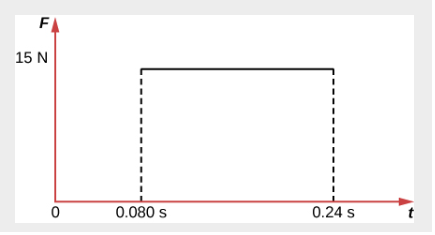
Force vs. time graph with horizontal line at 15 newtons between 0.080s and 0.24s. — Figure 1: This is a graph showing the force exerted by a fixed barrier on a block versus time.

$\Delta p=F \Delta t=(15 N)(0.24 \mathrm{~s})=3.6 \mathrm{~kg} \cdot \mathrm{m} / \mathrm{s}$

Note that the initial momentum of the block is

$p_{\text {initial }}=m v_{\text {initial }}=(1.2 \mathrm{~kg})\left(-\frac{3.0 \mathrm{~m}}{\mathrm{~s}}\right)=-3.6 \mathrm{~kg} \cdot \mathrm{m} / \mathrm{s}$

We are assuming that the initial velocity is −3.0 m/s. We have established that the force exerted by the barrier is in the positive direction, so the initial velocity of the block must be in the negative direction. Since the final momentum of the block is zero, the impulse is equal to the change in momentum of the block.

Suppose that, instead of striking a fixed barrier, the block is instead stopped by a spring. Consider the force exerted by the spring over the time interval from the beginning of the collision until the block comes to rest.

In this case, the impulse can be calculated again using the area under the curve (the area of a triangle):

$\Delta p=\frac{1}{2}(\text { base })(\text { height })=\frac{1}{2}(0.24 \mathrm{~s})(30 \mathrm{~N})=3.6 \mathrm{~kg} \cdot \mathrm{m} / \mathrm{s}$

Again, this is equal to the difference between the initial and final momentum of the block, so the impulse is equal to the change in momentum.

2. Calculating Magnitudes of Impulses – Two Billiard Balls Striking a Rigid Wall:

Two identical billiard balls strike a rigid wall with the same speed and are reflected without any change of speed. The first strikes perpendicular to the wall. The second ball strikes the wall at an angle of $30 °$ from the perpendicular and bounces off at an angle of $30 °$ from perpendicular to the wall.

(a) Determine the direction of force on the wall due to each ball.

(b) Calculate the ratio of the magnitudes of impulses on the two balls by the wall.

Answer:

Strategy for A: In order to determine the force on the wall, consider the force on the ball due to the wall using Newton’s second law and then apply Newton’s third law to determine the direction. Assume the x-axis to be normal to the wall and to be positive in the initial direction of motion. Choose the y-axis to be along the wall in the plane of the second ball’s motion. The momentum direction and the velocity direction are the same.

Solution for A: The first ball bounces directly into the wall and exerts a force on it in the +x direction. Therefore, the wall exerts a force on the ball in the −x direction. The second ball continues with the same momentum component in the y direction, but reverses its x-component of momentum, as seen by sketching a diagram of the angles involved and keeping in mind the proportionality between velocity and momentum.

These changes mean the change in momentum for both balls are in the −x direction, so the force of the wall on each ball is along the −x direction.

Strategy for B: Calculate the change in momentum for each ball, which is equal to the impulse imparted to the ball.

Solution for B: Let 𝑢 be the speed of each ball before and after collision with the wall, and 𝑚 the mass of each ball. Choose the x-axis and y-axis as previously described and consider the change in momentum of the first ball which strikes perpendicular to the wall.

$p_{x i}=m u ; p_{y i}=0$

$p_{x f}=-m u ; p_{y f}=0$

Impulse is the change in momentum vector. Therefore, the x-component of impulse is equal to −2𝑚𝑢 and the y-component of impulse is equal to zero.

Now consider the change in momentum of the second ball.

$p_{x i}=m u \cos 30^{\circ} ; p_{y i}=-m u \sin 30^{\circ}$

$p_{x f}=-m u \cos 30^{\circ} ; p_{y f}=-m u \sin 30^{\circ}$

It should be noted here that while $p_x$ changes sign after the collision, $p_y$ does not. Therefore, the x-component of impulse is equal to $- 2 m u \cos 30 °$ and the y-component of impulse is equal to zero. The ratio of the magnitudes of the impulse imparted to the balls is $\frac{2 m u}{2 m u \cos 30^{\circ}}=\frac{2}{\sqrt{3}}=1.155$

3. Making connections – baseball:

In most real-life collisions, the forces acting on an object are not constant. For example, when a bat strikes a baseball, the force is small at the beginning of the collision since only a small portion of the ball is initially in contact with the bat. As the collision continues, the ball deforms so that a greater fraction of the ball is in contact with the bat, resulting in a greater force. As the ball begins to leave the bat, the force drops to zero. Although the changing force is difficult to precisely calculate at each instant, the average force can be estimated very well in most cases.

Suppose that a 150-g baseball experiences an average force of 480 N in a direction opposite the initial 32 m/s speed of the baseball over a time interval of 0.017 s. What is the final velocity of the baseball after the collision?

$\Delta p=F \Delta t=(480)(0.017)=8.16 \mathrm{~kg} \cdot \mathrm{m} / \mathrm{s}$

$m v_f-m v_i=8.16 \mathrm{~kg} \cdot \mathrm{m} / \mathrm{s}$

$(0.150 \mathrm{~kg}) v_f-(0.150 \mathrm{~kg})(-32 \mathrm{~m} / \mathrm{s})=8.16 \mathrm{~kg} \cdot \mathrm{m} / \mathrm{s}$

$v_f=22 \mathrm{~m} / \mathrm{s}$

Conservation of Momentum

Momentum is an important quantity because it is conserved. Yet it was not conserved in the examples in Impulse and Linear Momentum and Force, where large changes in momentum were produced by forces acting on the system of interest. Under what circumstances is momentum conserved?

The answer to this question entails considering a sufficiently large system. It is always possible to find a larger system in which total momentum is constant, even if momentum changes for components of the system. If a football player runs into the goalpost in the end zone, there will be a force on him that causes him to bounce backward. However, the Earth also recoils —conserving momentum—because of the force applied to it through the goalpost. Because Earth is many orders of magnitude more massive than the player, its recoil is immeasurably small and can be neglected in any practical sense, but it is real, nevertheless.

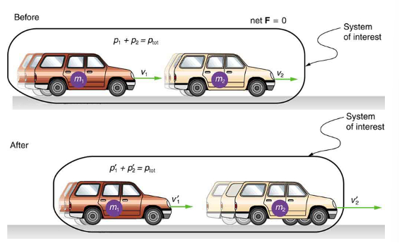
Consider what happens if the masses of two colliding objects are more similar than the masses of a football player and Earth – for example, one car bumping into another, as shown in Figure 2. Both cars are coating in the same direction when the lead car (labeled $m_2$ ) is bumped by the trailing car (labeled $m_1$ ). The only unbalanced force on each car is the force of the collision. (Assume that the effects due to friction are negligible). Car 1 slows down as a result of the collision, losing some momentum, while car 2 speeds up and gains some momentum. We shall now show that the total momentum of the two-car system remains constant.

Two images of cars traveling one behind the other. — Figure 2: A car of mass $m_1$ moving with a velocity of $\boldsymbol{v}_1$ bumps into another car of mass $m_2$ and velocity $v_2$ that it is following. As a result, the first car slows down to a velocity of $v_1^{\prime}$ and the second speeds up to a velocity of $v_2^{\prime}$ . The momentum of each car is changed, but the total momentum $p_{\text {tot }}$ of the two cars is the same before and after the collision (if you assume friction to be negligible)

Using the definition of impulse, the change in momentum of car 1 is given by

$\Delta p_1=F_1 \Delta t$ ,

where $F_1$ is the force on car 1 due to car 2, and $\Delta t$ is the time the force acts (the duration of the collision). Intuitively, it seems obvious that the collision time is the same for both cars, but it is only true for objects traveling at ordinary speeds. This assumption must be modified for objects travelling near the speed of light, without affecting the result that momentum is conserved.

Similarly, the change in momentum of car 2 is

$\Delta p_2=F_2 \Delta t$ ,

Where $F_2$ is the force on car 2 due to car 1, and we assume the duration of the collision $\Delta t$ is the same for both cars. We know from Newton’s third law that $F_2=-F_1$ , and so

$\Delta p_2=-F_1 \Delta t=-\Delta p_1$

Thus, the changes in momentum are equal and opposite, and

$\Delta p_1+\Delta p_2=0$

Because the changes in momentum add to zero, the total momentum of the two-car system is constant. That is,

$p_1+p_2=\text { constant }$ ,

$p_1+p_2=p_1^{\prime}+p_2^{\prime}$

Where $p_1^{\prime}{ }_1 \text { and } p_2^{\prime}$ are the momenta of cars 1 and 2 after the collision. (We often use primes to denote the final state.)

This result—that momentum is conserved—has validity far beyond the preceding one-dimensional case. It can be similarly shown that total momentum is conserved for any isolated system, with any number of objects in it. In equation form, the conservation of momentum principle for an isolated system is written

$p_{t o t}=\text { constant }$

Or

$p_{t o t}=p_{t o t}^{\prime}$

Where $p_{t o t}$ is the total momentum (the sum of the momenta of the individual objects in the system) and $p^{\prime}{ }_{t o t}$ is the total momentum some time later. (The total momentum can be shown to be the momentum of the center of mass of the system.) An isolated system is defined to be one for which the net external force is zero $\left(F_{\text {net }}=0\right)$

Elastic and Inelastic Collisions

Elastic Collisions in One Dimension

Let us consider several types of two-object collisions. These collisions are the easiest to analyze, and they illustrate many of the physical principles involved in collisions. The conservation of momentum principle is particularly useful here, and it can be used whenever the net external force on a system is zero.

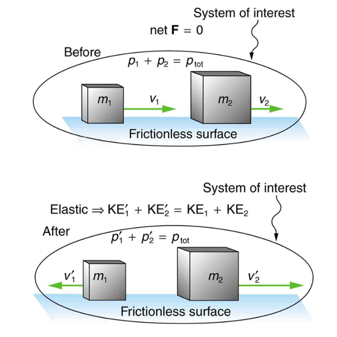
We start with the elastic collision of two objects moving along the same line—a one-dimensional problem. An elastic collision is one that also conserves internal kinetic energy. Internal kinetic energy is the sum of the kinetic energies of the objects in the system. Figure 3 below illustrates an elastic collision in which internal kinetic energy and momentum are conserved.

Truly elastic collisions can only be achieved with subatomic particles, such as electrons striking nuclei. Macroscopic collisions can be very nearly, but not quite, elastic—some kinetic energy is always converted into other forms of energy such as heat transfer due to friction and sound. One macroscopic collision that is nearly elastic is that of two steel blocks on ice. Another nearly elastic collision is that between two carts with spring bumpers on an air track. Icy surfaces and air tracks are nearly frictionless, more readily allowing nearly elastic collisions on them.

Two images of two blocks' motions. — Figure 3: *An elastic one-dimensional two-object collision. Momentum and internal kinetic energy are conserved.*

Now, to solve problems involving one-dimensional elastic collisions between two objects we can use the equations for conservation of momentum and conservation of internal kinetic energy. First, the equation for conservation of momentum for two objects in a one-dimensional collision is

$p_1+p_2=p_1^{\prime}+p_2^{\prime}\left(F_{\text {net }}=0\right)$

Or

$m_1 v_1+m_2 v_2=m_1 v^{\prime}{ }_1+m_2 v^{\prime}{ }_2\left(F_{\text {net }}=0\right)$

Where the primes (‘) indicate values after the collision. By definition, an elastic collision conserves internal kinetic energy, and so the sum of kinetic energies before the collision equals the sum after the collision. Thus,

$\frac{1}{2} m_1 v_1^2+\frac{1}{2} m_2 v_2^2=\frac{1}{2} m_1 v_1^{\prime 2}+\frac{1}{2} m_2 v_2^{\prime 2}(\text { two }-\text { object elastic collision })$

Expresses the equation for conservation of internal kinetic energy in a one-dimensional collision.

Example 4

Calculating velocities following an elastic collision:

Calculate the velocities of two objects following an elastic collision, given that

$m_1=0.500 \mathrm{~kg}, m_2=3.50 \mathrm{~kg}, v_1=4.00 \frac{\mathrm{m}}{\mathrm{s}}, v_2=0$ .

Answer: For this problem, note that $v_2=0$ and use conservation of momentum.

Thus, $p_1=p_1^{\prime}+p_2^{\prime} \text { or } m_1 v_1=m_1 v_1^{\prime}+m_2 v_2^{\prime}$

Using conservation of internal kinetic energy and that $v_2=0$ ,

$\frac{1}{2} m_1 v_1^2=\frac{1}{2} m_1 v_1^{\prime 2}+\frac{1}{2} m_2 v_2^{\prime 2}$

Solving the first equation (momentum equation) for $v_2^{\prime}, \text { we obtain }$

$v_2^{\prime}=\frac{m_1}{m_2}\left(v_1-v_1^{\prime}\right)$ .

Substituting this expression into the second equation (internal kinetic energy equation) eliminates the variable ${v'}_{2}$ leaving only $v_1^{\prime}$ as an unknown. There are two solutions to any quadratic equation; in this example, they are $v_1^{\prime}=4.00 \mathrm{~m} / \mathrm{s}$ and $v^{\prime} 1=-3.00 \mathrm{~m} / \mathrm{s}$ . Both solutions may or may not be meaningful. In this case, the first solution is the same as the initial condition. The first solution thus represents the situation before the collision is discarded. The second solution $\left(v^{\prime}{ }_1=-3.00 \mathrm{~m} / \mathrm{s}\right)$ is negative, meaning that the first object bounces backward. When this negative value of $v_1^{\prime}$ is used to find the velocity of the second object after the collision, we get

$v_2^{\prime}=\frac{m_1}{m_2}\left(v_1-v^{\prime}{ }_1\right)=\frac{0.500 \mathrm{~kg}}{3.50 \mathrm{~kg}}[4.00-(-3.00)] \mathrm{m} / \mathrm{s}$

$v_2^{\prime}=1.00 \mathrm{~m} / \mathrm{s}$

Collision Lab – PhET Simulation

Inelastic Collisions in One Dimension

We have seen that in an elastic collision, internal kinetic energy is conserved. An inelastic collision is one in which the internal kinetic energy changes (it is not conserved). This lack of conservation means that the forces between colliding objects may remove or add internal kinetic energy. Work done by internal forces may change the forms of energy within a system. For inelastic collisions, such as when colliding objects stick together, this internal work may transform some internal kinetic energy into heat transfer. Or it may convert stored energy into internal kinetic energy, such as when exploding bolts separate a satellite from its launch vehicle.

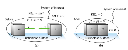
Figure 4 below shows an example of an inelastic collision. Two objects that have equal masses head toward one another at equal speeds and then stick together. Their total internal kinetic energy is initially $\frac{1}{2} m v^2+\frac{1}{2} m v^2=m v^2$ . The two objects come to rest after sticking together, conserving momentum. But the internal kinetic energy is zero after the collision. A collision in which the objects stick together is something called a perfectly inelastic collision because it reduces internal kinetic energy more than does any other type of inelastic collision. In fact, such a collision reduces internal kinetic energy to the minimum it can have while still conserving momentum.

Perfectly inelastic collision – a collision in which the objects stick together is sometimes called “perfectly inelastic.”

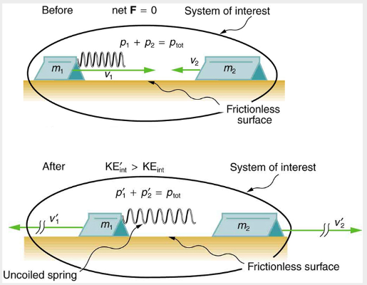
Example 5

Calculating final velocity and energy release – two carts collide:

In the collision pictured below in Figure 5, two carts collide inelastically. Cart 1 (denoted $m_1$ carries a spring which is initially compressed. During the collision, the spring releases its potential energy and converts it to internal kinetic energy. The mass of cart 1 and the spring is $0.350 \mathrm{~kg}$ , and the cart and the spring together have an initial velocity of $2.00 \mathrm{~m} / \mathrm{s}$ . Cart 2 (denoted $\left.m_2\right)$ has a mass of 0.500 kg and an initial velocity of -0.500m/s. After the collision, cart 1 is observed to recoil with a velocity of -4.00m/s.

(a) What is the final velocity of cart 2?

(b) How much energy was released by the spring (assuming all of it was converted into internal kinetic energy)?

Answer:

(a) the equation for conservation of momentum in a two-object system is $m_1 v_1+m_2 v_2=m_1 v_1^{\prime}+m_2 v_2^{\prime}$ .

The only unknown in this equation is $v_2^{\prime}$ . Solving for $v_2^{\prime}$ and substituting known values into the previous equation yields.

$v_2^{\prime}=\frac{m_1 v_1+m_2 v_2-m_1 v_1^{\prime}}{m_2}$

$=\frac{(0.350 \mathrm{~kg})(2.00 \mathrm{~m} / \mathrm{s})+(0.500 \mathrm{~kg})(-0.500 \mathrm{~m} / \mathrm{s})}{0.500 \mathrm{~kg}}-\frac{(0.350 \mathrm{~kg})(-4.00 \mathrm{~m} / \mathrm{s})}{0.500 \mathrm{~kg}}$

$=3.70 \mathrm{~m} / \mathrm{s}$

(b) the internal kinetic energy before the collision is

$K E_{i n t}=\frac{1}{2} m_1 v_1^2+\frac{1}{2} m_2 v_2^2$

$=\frac{1}{2}(0.350 \mathrm{~kg})(2.00 \mathrm{~m} / \mathrm{s})^2+\frac{1}{2}(0.500 \mathrm{~kg})(-0.500 \mathrm{~m} / \mathrm{s})^2$

$=0.763 \mathrm{~J}$

After the collision, the internal kinetic energy is

$K E^{\prime}{ }_{i n t}=\frac{1}{2} m_1 v_1^{\prime 2}+\frac{1}{2} m_2 v_2^{\prime}{ }_2^2$

$=\frac{1}{2}(0.350 \mathrm{~kg})(-4.00 \mathrm{~m} / \mathrm{s})^2+\frac{1}{2}(0.500 \mathrm{~kg})(3.70 \mathrm{~m} / \mathrm{s})^2$

$=6.22 \mathrm{~J}$

The change in internal kinetic energy is thus

$K E_{i n t}^{\prime}-K E_{i n t}=6.22 J-0.763 J=5.46 J$

Collisions of Point Masses in Two Dimensions

In the previous two sections, we considered only one-dimensional collisions; during such collisions, the incoming and outgoing velocities are all along the same line. But what about collisions, such as those between billiard balls, in which objects scatter to the side? These are two-dimensional collisions, and we shall see that their study is an extension of the one-dimensional analysis already presented. The approach taken (similar to the approach in discussing two-dimensional kinematics and dynamics) is to choose a convenient coordinate system and resolve the motion into components along perpendicular axes. Resolving the motion yields a pair of one-dimensional problems to be solved simultaneously.

One complication arising in two-dimensional collisions is that the objects might rotate before or after their collision. For example, if two ice skaters hook arms as they pass by one another, they will spin in circles. To avoid rotation, we consider only the scattering of point masses – that is, structureless particles that cannot rotate or spin.

We start by assuming that $F_{\text {net }}=0$ , so that momentum p is conserved. The simplest collision is one in which one of the particles is initially at rest. See Figure 4 below. The best choice for a coordinate system is one with an axis parallel to the velocity of the incoming particle, as shown in Figure 6. Because momentum is conserved, the components of momentum along the x- and y- axes $\left(p_x \text { and } p_y\right)$ will also be conserved, but with the chosen coordinate system, $p_y$ is initially zero and $p_x$ is the momentum of the incoming particle. Both facts simplify the analysis. (Even with the simplifying assumptions of point masses, one particle initially at rest, and a convenient coordinate system, we still gain new insights into nature from the analysis of two-dimensional collisions.)

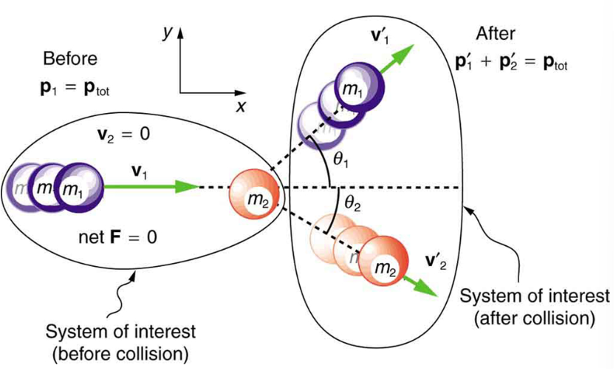Cartoon of billiard balls movements. — Figure 6: *A two-dimensional collision with the coordinate system chosen so that $m_2$* *is initially at rest and $v_1$* is parallel to the x -axis. This coordinate system is sometimes called the laboratory coordinate system, because many scattering experiments have a target that is stationary in the laboratory, while particles are scattered from it to determine the particles that make-up the target and how they are bound together. The particles may not be observed directly, but their initial and final velocities are.

Along the x-axis, the equation for conservation of momentum is

$p_{1 x}+p_{2 x}=p^{\prime}{ }_{1 x}+p^{\prime}{ }_{2 x}$

Where the subscripts denote the particles and axes, and the primes denote the situation after the collision. In terms of masses and velocities, this equation is

$m_1 v_{1 x}+m_2 v_{2 x}=m_1 v_{1 x}^{\prime}+m_2 v_{2 x}^{\prime}$

But because particle 2 is initially at rest, this equation becomes

$m_1 v_{1 x}=m_1 v_{1 x}^{\prime}+m_2 v_{2 x}^{\prime}$

The components of the velocities along the x-axis have the form $v \cos \theta$ . Because particle 1 initially moves along the x-axis, we find $v_{1 x}=v_1$ .

Conservation of momentum along the x-axis gives the following equation:

$m_1 v_{1 x}=m_1 v_1^{\prime}{ }_1 \cos \theta_1+m_2 v_2^{\prime} \cos \theta_2$

Where $\theta_1 \text { and } \theta_2$ are shown in Figure 4.

Along the y-axis, the equation for conservation of momentum is

$p_{1 y}+p_{2 y}=p_{1 y}+p_{2 y}$

Or

$m_1 v_{1 y}+m_2 v_{2 y}=m_1 v_{1 y}^{\prime}+m_2 v_{2 y}^{\prime}$

But $v_{1 y}$ is zero, because particle 1 initially moves along the x-axis. Because particle 2 is initially at rest, $v_{2 y}$ is also zero. The equation for conservation of momentum along the y-axis becomes

$0=m_1 v_{1 y}^{\prime}+m_2 v_{2 y}^{\prime}$

The components of the velocities along the y-axis have the form $v \sin \theta$ . Thus, the conservation of momentum along the y-axis gives the following equation:

$0=m_1 v_1^{\prime}{ }_1 \sin \theta_1+m_2 v_2^{\prime} \sin \theta_2$

Making Connections: Real World Connections

We have seen, in one-dimensional collisions when momentum is conserved, that the center-of-mass velocity of the system remains unchanged as a result of the collision. If you calculate the momentum and center-of-mass velocity before the collision, you will get the same answer as if you calculate both quantities after the collision. This logic also works for two-dimensional collisions.

For example, consider two cars of equal mass. Car A is driving east (+x-direction) with a speed of 40 m/s. Car B is driving north (+y-direction) with a speed of 80 m/s. What is the velocity of the center-of-mass of this system before and after an inelastic collision, in which the cars move together as one mass after the collision?

Since both cars have equal mass, the center-of-mass velocity components are just the average of the components of the individual velocities before the collision. The x-component of the center of mass velocity is 20 m/s, and the y-component is 40 m/s.

Using momentum conservation for the collision in both the x-component and y-component yields similar answers:

$m(40)+m(0)=(2 m) v_{\text {final }}(x)$

$v_{\text {final }}(x)=20 \mathrm{~m} / \mathrm{s}$

$m(0)+m(80)=(2 m) v_{\text {final }}(y)$

$v_{\text {final }}(y)=40 \mathrm{~m} / \mathrm{s}$

Since the two masses move together after the collision, the velocity of this combined object is equal to the center-of-mass velocity. Thus, the center-of-mass velocity before and after the collision is identical, even in two-dimensional collisions, when momentum is conserved.

Elastic and Inelastic Collisions

Deriving the Shortcut to Solve Elastic Collision Problems

How to Use the Shortcut for Solving Elastic Collisions

Balance Forces on a Stationary Object in Equilibrium

Equilibrium Forces

Check Your Understanding: Equilibrium Forces

Static Equilibrium

Balancing Act PhET Simulation

The First Condition for Equilibrium

The first condition necessary to achieve equilibrium is that the net external force on the system must be zero. Expressed as an equation, this is simply

$\text { net } F=0$

Note that if net F is zero, then the net external force in any direction is zero. For example, the net external forces along the typical x- and y-axes are zero. This is written as $\text { net } F_x=0 \text { and } F_y=0$ .

The Second Condition for Equilibrium

The second condition necessary to achieve equilibrium involves avoiding accelerated rotation (maintaining a constant angular velocity). A rotating body or system can be in equilibrium if its rate of rotation is constant and remains unchanged by the forces acting on it. The magnitude, direction, and point of application of the force are incorporated into the definition of the physical quantity called torque.

Torque is the rotational equivalent of a force. It is a measure of the effectiveness of a force in changing or accelerating a rotation (changing the angular velocity over a period of time). In equation form, the magnitude of torque is defined to be

$\tau=r F \sin (\theta)$

Where $\tau$ is the symbol for torque, r is the distance from the pivot point to the point where the force is applied, F is the magnitude of the force, and $\theta$ is the angle between the force and the vector directed from the point of application to the pivot point.

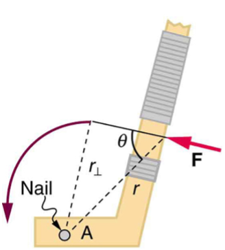
An object showing the three factors for a pivot point. — Figure 7: A force applied to an object can produce a torque, which depends on the location of the pivot point. The three factors $r, F \text {, and } \theta$ for pivot point A on a body are shown here – r is the distance from the chosen pivot point to the point where the force F is applied, and $\theta$ is the angle between F and the vector directed from the point of application to the pivot point. If the object can rotate around point A, it will rotate counterclockwise. This means that torque is counterclockwise relative to pivot A.

Figure 7: A force applied to an object can produce a torque, which depends on the location of the pivot point. The three factors $r, F \text {, and } \theta$ for pivot point A on a body are shown here – r is the distance from the chosen pivot point to the point where the force F is applied, and $\theta$ is the angle between F and the vector directed from the point of application to the pivot point. If the object can rotate around point A, it will rotate counterclockwise. This means that torque is counterclockwise relative to pivot A.

The perpendicular lever arm $r_{\perp}$ is the shortest distance from the pivot point to the line along which F acts; it is shown as a dashed line in Figure 7. Note that the line segment that defines the distance $r_{\perp}$ is perpendicular to F, as its name implies. It is sometimes easier to find or visualize $r_{\perp}$ than to find both r and $\theta$ . In such cases, it may be more convenient to use $\tau=r_{\perp} F$ rather than $\tau=r F \sin (\theta)$ for torque, but both are equally valid.

The SI unit of torque is newtons time meters, usually written as $N \cdot m$ . For example, if you push perpendicular to the door with a force of 40 N at a distance of 0.800 m from the hinges, you exert a torque of $32 N \cdot m\left(0.800 m \times 40 N \times \sin \left(90^{\circ}\right)\right.$ relative to the hinges. If you reduce the force to 20 N, the torque is reduced to $16 N \cdot m$ , and so on.

Now, the second condition necessary to achieve equilibrium is that the net external torque on a system must be zero. An external torque is one that is created by an external force. You can choose the point around which the torque is calculated. The point can be the physical pivot point of a system or any other point in space—but it must be the same point for all torques. If the second condition (net external torque on a system is zero) is satisfied for one choice of pivot point, it will also hold true for any other choice of pivot point in or out of the system of interest. (This is true only in an inertial frame of reference.) The second condition necessary to achieve equilibrium is stated in equation form as $\text { net } \tau=0$ where net means total. Torques, which are in opposite directions are assigned opposite signs. A common convention is to call counterclockwise (ccw) torques positive and clockwise (cw) torques negative.

When two children balance a seesaw as shown in Figure 8, they satisfy the two conditions for equilibrium. Most people have perfect intuition about seesaws, knowing that the lighter child must sit farther from the pivot and that a heavier child can keep a lighter one off the ground indefinitely.

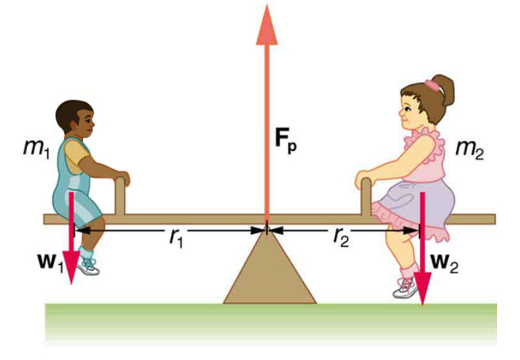
Cartoon of two children balancing on a seesaw. — Figure 8: Two children balancing a seesaw satisfy both conditions for equilibrium. The lighter child sits farther from the pivot to create a torque equal in magnitude to that of the heavier child.

Example 6

The two children shown in Figure 8 above are balanced on a seesaw of negligible mass. (This assumption is made to keep the example simple). The first child has a mass of 26.0 kg and sits 1.60 m from the pivot. (a) If the second child has a mass of 32.0 kg, how far is she from the pivot? (b) What is $F_p$ the supporting force exerted by the pivot?

Strategy:

Both conditions for equilibrium must be satisfied. In part (a), we are asked for a distance; thus, the second condition (regarding torques) must be used, since the first (regarding only forces) has no distances in it. To apply the second condition for equilibrium, we first identify the system of interest to be the seesaw plus the two children. We take the supporting pivot to be the point about which the torques are calculated. We then identify all external forces acting on the system.

Solution (a)

The three external forces acting on the system are the weights of the two children and the supporting force of the pivot. Let us examine the torque produced by each. Torque is defined to be

$\tau=r F \sin (\theta)$

Here $\theta=90^{\circ}$ , so that $\sin (\theta)=1$ for all three forces. That means $\tau_{\perp}=r$ for all three. The torques exerted by the three forces are first,

$\tau_1=r_1 w_1$

Second,

$\tau_2=-r_2 w_2$

And third,

$\tau_p=r_p F_p$

$=0 \cdot F_p$

= 0

Note that a minus sign has been inserted into the second question because this torque is clockwise and is therefore negative by convention. Since $F_p$ act directly on the pivot point, the distance $r_p$ is zero. A force acting on the pivot cannot cause a rotation, just as pushing directly on the hinges of a door will not cause it to rotate. Now, the second condition for equilibrium is that the sum of the torques on both children is zero. Therefore

$\tau_2=-\tau_1$

Or

$r_2 w_2=r_1 w_1$

Weight is mass times the acceleration due to gravity. Entering mg for w, we get

$r_2 m_2 g=r_1 m_1 g$

Solve this for the unknown $r_2$ :

$r_2=r_1 \frac{m_1}{m_2}$

The quantities on the right side of the equation are known; thus, $r_2$ is

$r_2=(1.60 \mathrm{~m}) \frac{26.0 \mathrm{~kg}}{32.0 \mathrm{~kg}}=1.30 \mathrm{~m}$

As expected, the heavier child must sit closer to the pivot (1.30 m versus 1.60 m) to balance the seesaw.

Solution (b)

This part asks for a force $F_p$ . The easiest way to find it is to use the first condition for equilibrium, which is

$\text { net } F=0$

The forces are all vertical, so that means we are dealing with a one-dimension problem along the vertical axis; hence, the condition can be written as

$\text { net } F_y=0$

Where we again call the vertical axis the y-axis. Choosing upward to be the positive direction, and using plus and minus signs to indicate the directions of the forces, we see that

$F_p-w_1-w_2=0$

This equation yields what might have been guessed at the beginning:

$F_p=w_1+w_2$

So, the pivot supplies a supporting force equal to the total weight of the system:

$F_p=m_1 g+m_2 g$

Entering known values gives

$F_p=(26.0 \mathrm{~kg})\left(9.80 \mathrm{~m} / \mathrm{s}^2\right)+(32.0 \mathrm{~kg})\left(9.80 \mathrm{~m} / \mathrm{s}^2\right)$

$=568 N$

Discussion:

The two results make intuitive sense. The heavier child sits closer to the pivot. The pivot supports the weight of the two children. Part (b) can also be solved using the second condition for equilibrium, since both distances are known, but only if the pivot point is chosen to be somewhere other than the location of the seesaw’s actual pivot!

Several aspects of the preceding example have broad implications. First, the choice of the pivot as the point around which torques are calculated simplified the problem. Since $F_p$ is exerted on the pivot point, its lever arm is zero. Hence, the torque exerted by the supporting force $F_p$ is zero relative to that pivot point. The second condition for equilibrium holds for any choice of pivot point, and so we choose the pivot point to simplify the solution of the problem.

Second, the acceleration due to gravity canceled in this problem, and we were left with a ratio of masses. This will not always be the case. Always enter the correct forces – do not jump ahead to enter some ratio of masses.

Third, the weight of each child is distributed over an area of the seesaw, yet we treated the weights as if each force were exerted at a single point. This is not an approximation – the distances $r_1 \text { and } r_2$ are the distances to points directly below the center of gravity of each child.

Finally, not that the concept of torque has an importance beyond static equilibrium. Torque plays the same role in rotational motion that force plays in linear motion.

Stability

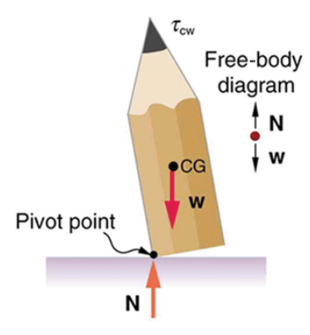
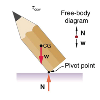
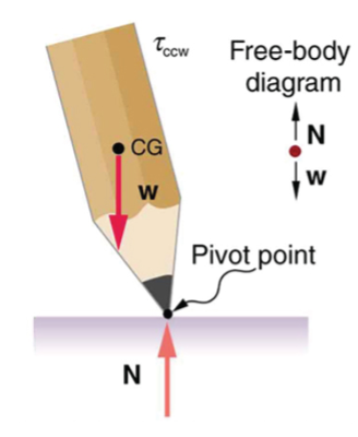
A system is said to be in stable equilibrium if, when displaced from equilibrium, it experiences a net force or torque in a direction opposite to the direction of the displacement. For example, a marble at the bottom of a bowl will experience a restoring force when displaced from its equilibrium position. This force moves it back toward the equilibrium position. Most systems are in stable equilibrium, especially for small displacements. For another example of stable equilibrium, see the pencil in Figure 9.

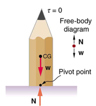
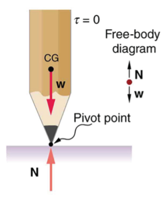
Pencil with a freebody diagram. The normal force points N and the weight points S — Figure 9: This pencil is in the condition of equilibrium. The net force on the pencil is zero and the total torque about any pivot is zero.

A system is in unstable equilibrium if, when displaced, it experiences a net force or torque in the same direction as the displacement from equilibrium. A system in unstable equilibrium accelerates away from its equilibrium position if displaced even slightly. An obvious example is a ball resting on top of a hill. Once displaced, it accelerates away from the crest. See Figures 10-13 for examples of unstable equilibrium.

Pencil tilting slightly to the left. Normal force points N and weight points S. — Figure 10: If the pencil is displaced slightly to the side (counterclockwise), it is no longer in equilibrium. Its weight produces a clockwise torque that returns the pencil to its equilibrium position.

Pencil tilting to the left. Normal force points N and the weight points S. — Figure 11: If the pencil is displaced too far, the torque caused by its weight changes to counterclockwise and causes the displacement to increase.

Pencil tip down. Normal force points N and weight points S. — Figure 12: This figure shows unstable equilibrium, although both conditions for equilibrium are satisfied.

Pencil tip down tilting slightly left. Normal force points N and weight points S. — Figure 13: If the pencil is displaced even slightly, a torque is created by its weight that is in the same direction as the displacement, causing the displacement to increase.

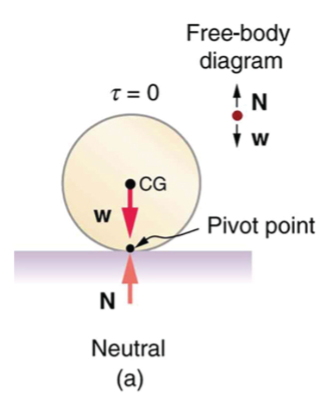
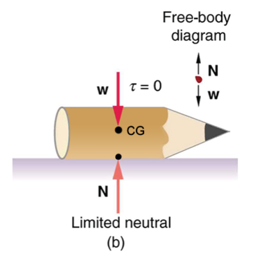
A system is in neutral equilibrium if its equilibrium is independent of displacements from its original position. A marble on a flat horizontal surface is an example. Combinations of these situations are possible. For example, a marble on a saddle is stable for displacements toward the front or back of the saddle and unstable for displacements to the side. Figures 14-15 show another example of neutral equilibrium.

Ball at neutral position with normal force pointing N and weight pointing S. — Figure 14: Here we see neutral equilibrium. The cg of a sphere on a flat surface lies directly above the point of support, independent of the position on the surface. The sphere is therefore in equilibrium in any location, and if displaced, it will remain put.

Pencil on its side. Normal force points N and weight points S. — Figure 15: Because it has a circular cross section, the pencil is in neutral equilibrium for displacements perpendicular to its length.

Center of Gravity

Dynamic Balance

Check Your Understanding: Stability

Relevance to Transportation Engineering Coursework

This section explains the relevance of traffic safety and superelevation to transportation engineering coursework.

Traffic Safety

Avoiding collisions (or crashes) and in case collisions do occur minimization of harm to human beings involved are of critical importance in transportation engineering practice. Practitioners and researchers recommend use of term “crashes” or “collisions” instead of “accidents” so that they are thought of as preventable events instead of inevitable incidents with no possible avoidance/mitigation measures. Crashes are classified according to their severity from property-damage-only (PDO) to fatal, and the crash severity is highly correlated with the impact speed, and hence the momentum. Mitigation measures, such as guardrails, traffic signs with breakaway poles, crash attenuators, air bags, seat belts, and child seats are all implemented to reduce the severities of crashes according to the momentum principles, described in the section titled “Use of Momentum Preservation to Describe the Post-Collision Movement of Objects.”

Superelevation

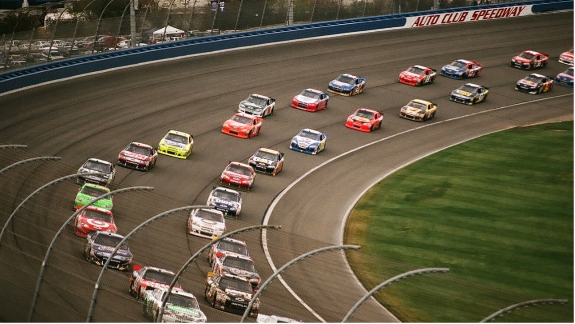
Superelevation, i.e., raising of outer edge of the pavement relative to the inner edge, is provided to support higher speed travel along a horizontal curve. The banking helps provide the required inward force to keep vehicle on a circular motion. Figure 14 illustrates a superelevated curved segment of racetrack, where the relative elevation of the outer edge is more pronounced (compared to public roadways) due to significantly higher speeds of race cars. The formula for estimating the required superelevation for a given design speed is based on the principles of balancing forces described in the above section titled “Balance Forces on a Stationary Object in Equilibrium.”

Nascar Yellow Flag Lineup — Figure 16: Superelevated segment of a racetrack with raised outer edge

Key Takeaways

Transportation engineers and safety professionals recognize that crashes and collisions are not “accidents” in the sense that these events are not inevitable, can be prevented, and their impacts can be mitigated. One key aspect of crash impact mitigation is to reduce the severity of collisions that do occur, especially those involving VRUs. The speed-momentum relationships discussed in this chapter are essential to developing this understanding.
Superelevation or banking refers to the raised outer edge of a roadway segment on a horizontal curve. It is provided to counteract the tendency of a vehicle to roll outward on a curve. With a gravitational force component pulling the vehicle inward, the superelevation helps keep the vehicle on a circular path providing stability and control for negotiating circular curve segments at higher speeds.

Glossary: Key Terms

Center of Gravity[1] – the point where the total weight of the body is assumed to be concentrated

Change in Momentum[1]– the difference between the final and initial momentum; the mass times the change in velocity

Conservation of Momentum Principle[1] – when the net external force is zero, the total momentum of the system is conserved or constant

Dynamic Equilibrium[1] – a state of equilibrium in which the net external force and torque on a system moving with constant velocity are zero

Elastic Collision[1] – a collision that also conserves internal kinetic energy

Impulse[1] – the average net external force times the time it acts; equal to the change in momentum

Inelastic Collision[1] – a collision in which internal kinetic energy is not conserved

Internal Kinetic Energy[1] – the sum of the kinetic energies of the objects in a system

Isolated System[1] – a system in which the net external force is zero

Linear Momentum[1] – the product of mass and velocity

Neutral Equilibrium[1] – a state of equilibrium that is independent of a system’s displacements from its original position

Perfectly Inelastic Collision[1] – a collision in which the colliding objects stick together

Perpendicular Lever Arm[1] – the shortest distance from the pivot point to the line along which 𝐹 lies

Point Masses[1] – structureless particles with no rotation or spin

Second Law of Motion[1] – physical law that states that the net external force equals the change in momentum of a system divided by the time over which it changes

SI Units of Torque[1]– newton times meters, usually written as 𝑁∙𝑚

Stable Equilibrium[1] – a system, when displaced, experiences a net force or torque in a direction opposite to the direction of the displacement

Static Equilibrium[1] – a state of equilibrium in which the net external force and torque acting on a system is zero; equilibrium in which the acceleration of the system is zero and accelerated rotation does not occur

Torque[1] – turning or twisting effectiveness of a force

Unstable Equilibrium[1] – a system, when displaced, experiences a net force or torque in the same direction as the displacement from equilibrium

[1] “College Physics for AP® Courses” by Greg Wolfe, Erika Gasper, John Stoke, Julie Kretchman, David Anderson, Nathan Czuba, Sudhi Oberoi, Liza Pujji, Irina Lyublinskaya, Douglas Ingram. Access for free at https://openstax.org/books/college-physics-ap-courses/pages/1-connection-for-ap-r-courses

Media Attributions

Note: All Khan Academy content is available for free at (www.khanacademy.org).

Note: Text by Greg Wolfe, et al.: Access for free at https://openstax.org/books/college-physics-ap-courses/pages/1-connection-for-ap-r-courses

videos

Video 1: Introduction to Momentum by Khan Academy is licensed by Creative Commons NonCommercial-ShareAlike 3.0 United States (CC BY-NC-SA 3.0 US)
Video 2: Impulse and Momentum Dodgeball Example by Khan Academy is licensed by Creative Commons NonCommercial-ShareAlike 3.0 United States (CC BY-NC-SA 3.0 US)
Video 3: Bouncing Fruit Collision Example by Khan Academy is licensed by Creative Commons NonCommercial-ShareAlike 3.0 United States (CC BY-NC-SA 3.0 US)
Video 4: Momentum: Ice Skater Throws a Ball by Khan Academy is licensed by Creative Commons NonCommercial-ShareAlike 3.0 United States (CC BY-NC-SA 3.0 US)
Video 5: 2-Dimensional Momentum Problem by Khan Academy is licensed by Creative Commons NonCommercial-ShareAlike 3.0 United States (CC BY-NC-SA 3.0 US)
Video 6: Part 2 by Khan Academy is licensed by Creative Commons NonCommercial-ShareAlike 3.0 United States (CC BY-NC-SA 3.0 US)
Video 7: Force vs. Time Graphs by Khan Academy is licensed by Creative Commons NonCommercial-ShareAlike 3.0 United States (CC BY-NC-SA 3.0 US)
Video 8: Momentum Notes by Jeff Batey is licensed by Creative Commons Attribution 3.0 Unported (CC BY 3.0)
Video 9: Elastic and Inelastic Collisions by Khan Academy is licensed by Creative Commons NonCommercial-ShareAlike 3.0 United States (CC BY-NC-SA 3.0 US)
Video 10: Deriving the Shortcut to Solve Elastic Collision Problems by Khan Academy is licensed by Creative Commons NonCommercial-ShareAlike 3.0 United States (CC BY-NC-SA 3.0 US)
Video 11: How to Use the Shortcut for Solving Elastic Collisions by Khan Academy is licensed by Creative Commons NonCommercial-ShareAlike 3.0 United States (CC BY-NC-SA 3.0 US)
Video 12: Equilibrium Forces by Jennifer Cash is licensed by Creative Commons Attribution 3.0 Unported (CC BY 3.0)
Video 13: Static Equilibrium by Jennifer Cash is licensed by Creative Commons Attribution 3.0 Unported (CC BY 3.0)
Video 14: Center of Gravity by Jennifer Cash is licensed by Creative Commons Attribution 3.0 Unported (CC BY 3.0)
Video 15: Dynamic Balance by Alejandro Garcia is licensed by Creative Commons Attribution 3.0 Unported (CC BY 3.0)

figures

Figure 1: “College Physics for AP® Courses” by Greg Wolfe, Erika Gasper, John Stoke, Julie Kretchman, David Anderson, Nathan Czuba, Sudhi Oberoi, Liza Pujji, Irina Lyublinskaya, Douglas Ingram is licensed by Creative Commons Attribution 4.0 International (CC BY 4.0). Access for free.
Figure 2: “College Physics for AP® Courses” by Greg Wolfe, Erika Gasper, John Stoke, Julie Kretchman, David Anderson, Nathan Czuba, Sudhi Oberoi, Liza Pujji, Irina Lyublinskaya, Douglas Ingram is licensed by Creative Commons Attribution 4.0 International (CC BY 4.0). Access for free.
Figure 3: “College Physics for AP® Courses” by Greg Wolfe, Erika Gasper, John Stoke, Julie Kretchman, David Anderson, Nathan Czuba, Sudhi Oberoi, Liza Pujji, Irina Lyublinskaya, Douglas Ingram is licensed by Creative Commons Attribution 4.0 International (CC BY 4.0). Access for free.
Figure 4: “College Physics for AP® Courses” by Greg Wolfe, Erika Gasper, John Stoke, Julie Kretchman, David Anderson, Nathan Czuba, Sudhi Oberoi, Liza Pujji, Irina Lyublinskaya, Douglas Ingram is licensed by Creative Commons Attribution 4.0 International (CC BY 4.0). Access for free.
Figure 5: “College Physics for AP® Courses” by Greg Wolfe, Erika Gasper, John Stoke, Julie Kretchman, David Anderson, Nathan Czuba, Sudhi Oberoi, Liza Pujji, Irina Lyublinskaya, Douglas Ingram is licensed by Creative Commons Attribution 4.0 International (CC BY 4.0). Access for free.
Figure 6:“College Physics for AP® Courses” by Greg Wolfe, Erika Gasper, John Stoke, Julie Kretchman, David Anderson, Nathan Czuba, Sudhi Oberoi, Liza Pujji, Irina Lyublinskaya, Douglas Ingram is licensed by Creative Commons Attribution 4.0 International (CC BY 4.0). Access for free.
Figure 7: “College Physics for AP® Courses” by Greg Wolfe, Erika Gasper, John Stoke, Julie Kretchman, David Anderson, Nathan Czuba, Sudhi Oberoi, Liza Pujji, Irina Lyublinskaya, Douglas Ingram is licensed by Creative Commons Attribution 4.0 International (CC BY 4.0). Access for free.
Figure 8: “College Physics for AP® Courses” by Greg Wolfe, Erika Gasper, John Stoke, Julie Kretchman, David Anderson, Nathan Czuba, Sudhi Oberoi, Liza Pujji, Irina Lyublinskaya, Douglas Ingram is licensed by Creative Commons Attribution 4.0 International (CC BY 4.0). Access for free.
Figure 9: “College Physics for AP® Courses” by Greg Wolfe, Erika Gasper, John Stoke, Julie Kretchman, David Anderson, Nathan Czuba, Sudhi Oberoi, Liza Pujji, Irina Lyublinskaya, Douglas Ingram is licensed by Creative Commons Attribution 4.0 International (CC BY 4.0). Access for free.
Figure 10: “College Physics for AP® Courses” by Greg Wolfe, Erika Gasper, John Stoke, Julie Kretchman, David Anderson, Nathan Czuba, Sudhi Oberoi, Liza Pujji, Irina Lyublinskaya, Douglas Ingram is licensed by Creative Commons Attribution 4.0 International (CC BY 4.0). Access for free.
Figure 11: “College Physics for AP® Courses” by Greg Wolfe, Erika Gasper, John Stoke, Julie Kretchman, David Anderson, Nathan Czuba, Sudhi Oberoi, Liza Pujji, Irina Lyublinskaya, Douglas Ingram is licensed by Creative Commons Attribution 4.0 International (CC BY 4.0). Access for free.
Figure 12: “College Physics for AP® Courses” by Greg Wolfe, Erika Gasper, John Stoke, Julie Kretchman, David Anderson, Nathan Czuba, Sudhi Oberoi, Liza Pujji, Irina Lyublinskaya, Douglas Ingram is licensed by Creative Commons Attribution 4.0 International (CC BY 4.0). Access for free.
Figure 13: “College Physics for AP® Courses” by Greg Wolfe, Erika Gasper, John Stoke, Julie Kretchman, David Anderson, Nathan Czuba, Sudhi Oberoi, Liza Pujji, Irina Lyublinskaya, Douglas Ingram is licensed by Creative Commons Attribution 4.0 International (CC BY 4.0). Access for free.
Figure 14: “College Physics for AP® Courses” by Greg Wolfe, Erika Gasper, John Stoke, Julie Kretchman, David Anderson, Nathan Czuba, Sudhi Oberoi, Liza Pujji, Irina Lyublinskaya, Douglas Ingram is licensed by Creative Commons Attribution 4.0 International (CC BY 4.0). Access for free.
Figure 15: “College Physics for AP® Courses” by Greg Wolfe, Erika Gasper, John Stoke, Julie Kretchman, David Anderson, Nathan Czuba, Sudhi Oberoi, Liza Pujji, Irina Lyublinskaya, Douglas Ingram is licensed by Creative Commons Attribution 4.0 International (CC BY 4.0). Access for free.
Figure 16: “College Physics for AP® Courses” by Greg Wolfe, Erika Gasper, John Stoke, Julie Kretchman, David Anderson, Nathan Czuba, Sudhi Oberoi, Liza Pujji, Irina Lyublinskaya, Douglas Ingram is licensed by Creative Commons Attribution 4.0 International (CC BY 4.0). Access for free.
Figure 17 is licensed by Creative Commons CC0 1.0 Universal (CC0 1.0) Public Domain Dedication

References

Farid, A. (2022). Traffic Safety and Human Factor Considerations. Personal Collection of Ahmed Farid, California Polytechnic State University, San Luis Obispo, CA.
Farid, A. (2022). Highway Design. Personal Collection of Ahmed Farid, California Polytechnic State University, San Luis Obispo, CA.

License

Icon for the Creative Commons Attribution-NonCommercial-ShareAlike 4.0 International License

OERTransport: Fundamentals of Math, Physics, and Statistics for Future Transportation Professionals Copyright © by Anurag Pande, Ph.D. in Civil Engineering (Transportation); Peyton Ratto, Civil Engineering MS/MCRP; and Ahmed Farid, Ph.D. in Civil Engineering is licensed under a Creative Commons Attribution-NonCommercial-ShareAlike 4.0 International License, except where otherwise noted.

Use of Momentum Preservation to Describe the Post-Collision Movement of Objects

Introduction to Momentum

Impulse and Momentum Dodgeball Example

Bouncing Fruit Collision Example

Momentum: Ice Skater Throws a Ball

2-Dimensional Momentum Problem (Trig Review!)

Part 2

Force vs. Time Graphs

Momentum Notes – Overview

Linear Momentum

Impulse

Conservation of Momentum

Elastic and Inelastic Collisions

Elastic Collisions in One Dimension

Collision Lab – PhET Simulation

Inelastic Collisions in One Dimension

Collisions of Point Masses in Two Dimensions

Elastic and Inelastic Collisions

Elastic and Inelastic Collisions

Deriving the Shortcut to Solve Elastic Collision Problems

How to Use the Shortcut for Solving Elastic Collisions

Balance Forces on a Stationary Object in Equilibrium

Equilibrium Forces

Static Equilibrium

Balancing Act PhET Simulation

The First Condition for Equilibrium

The Second Condition for Equilibrium

Stability

Center of Gravity

Dynamic Balance

Relevance to Transportation Engineering Coursework

Traffic Safety

Superelevation

Glossary: Key Terms

Media Attributions

videos

figures

References

License

Share This Book