Chapter 8: Probability: Basic Principles and Distributions
This chapter discusses understanding the basic principles of probability because transportation system operations and planning are critically dependent on these basic principles. Several processes are modeled using probability distributions for real-valued random variables. These distributions include normal distribution for the speed of vehicles on the road, Poisson’s distribution for gaps in traffic on an uncongested facility, or negative binomial as a distribution for crash frequency on a roadway segment.
Learning Objectives
At the end of the chapter, the reader should be able to do the following:
- Use basic counting techniques (multiplication rule, combinations, permutations) to estimate probability and odds.
- Set up and work with distributions for discrete random variables, including Bernoulli, binomial, geometric, and Poisson distributions.
- Set up and work with distributions for continuous random variables, including uniform, normal and exponential distributions.
- Identify topics in the introductory transportation engineering courses that build on the concepts discussed in this chapter.
Use Basic Counting Techniques to Estimate Probability and Odds
This section will explain ways to estimate probability and odds with videos to help your understanding. Also, short problems to check your understanding are included.
Multiplication Rule
Multiplication Rule
The multiplication rule says: If there are n ways to perform action 1 and then by m ways to perform action 2, then there are  ways to perform action 1 followed by action 2.
Count Outcomes Using Tree Diagram
Check Your Understanding: Multiplication Rule
Permutations
Permutations
A permutation of a set is a particular ordering of its elements. For example, the set  has six permutations: abc, acb, bac, bca, cab, cba. We found the number of permutations by listing them all. We could have also found the number of permutations by using the multiplication rule. That is, there are 3 ways to pick the first element, then 2 ways for the second, and 1 for the third. This gives a total of
  permutations.
In general, the multiplication rule tells us that the number of permutations of a set of elements is

We also talk about the permutations of k things out of a set of n things.
Example: List all the permutations of 3 elements out of the set 
| abc | acb | bac | bca | cab | cba |
| abd | adb | bad | bda | dab | dba |
| acd | adc | cad | cda | dac | dca |
| bcd | bdc | cbd | cdb | dbc | dcb |
Note that abc and acb count as distinct permutations. That is, for permutations the order matters.
There are 24 permutations. Note that the multiplication rule would have told us there are  permutations without bothering to list them all.
Permutation Formula
Zero Factorial
Ways to Pick Officers – Example
Check Your Understanding: Permutations
Combinations
Combinations
In contrast to permutations, in combinations order does not matter: permutations are lists and combinations are sets.
Example: List all the combinations of 3 elements out of the set .
Answer: Such a combination is a collection of 3 elements without regard to order. So, abc and cab both represent the same combination. We can list all the combinations by listing all the subsets of exactly 3 elements.

There are only 4 combinations. Contrast this with the 24 permutations in the previous example. The factor of 6 comes because every combination of 3 things can be written in 6 different orders.
Introduction to Combinations
Combination Formula
Combination Example: 9 Card Hands
Check Your Understanding: Combinations
Permutations and Combinations Comparison
We will use the following notations.
 = number of permutations (list) of k distinct elements from a set of size n
 = number of combinations (subsets) of k elements from a set of size n
We emphasize that by the number of combinations of k elements we mean the number of subsets of size k.
These have the following notation and formulas:
Permutations: 
Combinations: 
The notation  is read “n choose k”. The formula for follows from the multiplication rule. It also implies the formula for because a subset of size k can be ordered in k! ways.
We can illustrate the relationship between permutations and combinations by lining up the results of the previous two examples.
Permutations: 
| abc | acb | bac | bca | cab | cba |
| abd | adb | bad | bda | dab | dba |
| acd | adc | cad | cda | dac | dca |
| bcd | bdc | cbd | cdb | bdc | dcb |
Combinations: 

Notice that each row in the permutations list consists of all 3! permutations of the corresponding set in the combinations list.
Check Your Understanding: Permutations and Combinations Comparison
Probability Using the Rules
The General Multiplication Rule
When we calculate probabilities involving one event AND another event occurring, we multiply their probabilities.
In some cases, the first event happening impacts the probability of the second event. We call these dependent events.
In other cases, the first event happening does not impact the probability of the seconds. We call these independent events.
Independent events: Flipping a coin twice
What is the probability of flipping a fair coin and getting “heads” twice in a row? That is, what is the probability of getting heads on the first flip AND heads on the second flip?
Imagine we had 100 people simulate this and flip a coin twice. On average, 50 people would get heads on the first flip, and then 25 of them would get heads again. So, 25 out of the original 100 people – or 1/4 of them – would get heads twice in a row.
The number of people we start with does not really matter. Theoretically, 1/2 of the original group will get heads, and 1/2 of that group will get heads again. To find a fraction of a fraction, we multiply.
We can represent this concept with a tree diagram like the one shown below in Figure 1.
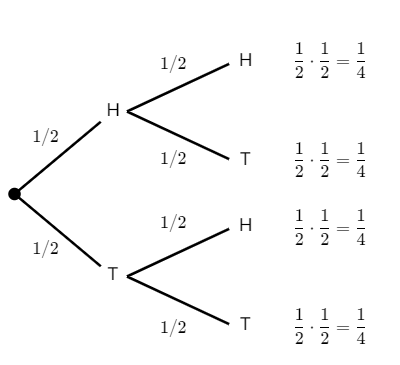
We multiply the probabilities along the branches to find the overall probability of one event AND the next event occurring.
For example, the probability of getting two “tails” in a row would be:

When two events are independent, we can say that

Be careful! This formula only applies to independent events.
Dependent events: Drawing cards
We can use a similar strategy even when we are dealing with dependent events.
Consider drawing two cards, without replacement, from a standard deck of 52 cards. That means we are drawing the first card, leaving it out, and then drawing the second card.
What is the probability that both cards selected are black?
Half of the 52 cards are black, so the probability that the first card is black is 26/52. But the probability of getting a black card changes on the next draw, since the number of black cards and the total number of cards have both been decreased by 1.
Here is what the probabilities would look like in a tree diagram:
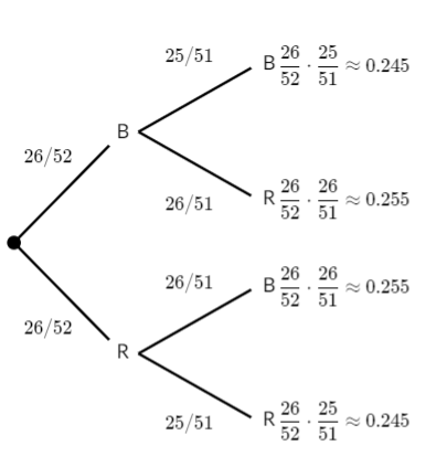
So, the probability that both cards are black is:

The General Multiplication Rule
For any two events, we can say that

The vertical bar in  means “given,” so this could also be read as “the probability that B occurs given that A has occurred.”
This formula says that we can multiply the probabilities of two events, but we need to take the first event into account when considering the probability of the second event.
If the events are independent, one happening does not impact the probability of the other, and in that case,  .
.
Check Your Understanding: Probability Using the Rules
Probability Using Combinations
Probability and Combinations
Conditional Probability and Bayes’ Theorem
Conditional Probability
Conditional probability answers the questions ‘how does the probability of an event change if we have extra information.’
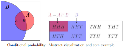
Example: Toss a fair coin 3 times.
What is the probability of 3 heads?
Answer: Sample space =  . All outcomes are equally likely, so
Suppose we are told that the first toss was heads. Given this information how should we compute the probability of 3 heads?
Answer: We have a new (reduced) sample space =  . All outcomes are equally likely, so
This is called conditional probability, since it takes into account additional conditions. To develop the notation, we rephrase (b) in terms of events.
Rephrased (b): Let A be the event ‘all three tosses are heads’ =  . Let B be the event ‘the first toss is heads’ = .
The conditional probability of A knowing that B occurred is written

This is read as ‘the conditional probability of A given B ’ OR ‘the probability of A conditioned on B ’ OR simply ‘the probability of A given B.’
We can visualize conditional probability as follows. Think of  as the proportion of the area of the whole sample space taken up by A. For we restrict our attention to B. That is, is the proportion of area of B taken up by A, i.e.,
  .
.
The formal definition of conditional probability catches the gist of the above example and visualization.
Formal definition of conditional probability
Let A and B be events. We define the conditional probability of A given B as

Let us redo the coin-tossing example using the definition in the equation above. Recall A = 3 heads and B = first toss is heads. We have  and
and  . Since
  , we also have
  . Now according to the equation,
  which agrees with the answer in Example B.
Bayes’ Theorem
Bayes’ theorem is a pillar of both probability and statistics. For two events A and B Bayes’ theorem says

Bayes’ rule tells us how to ‘invert’ conditional probabilities, i.e., to find from .
Proof of Bayes’ Theorem
The key point is that  is symmetric in A and B. So, the multiplication rule says
  .
.
Now divide through by P (A) to get Bayes’ rule.
A common mistake is to confuse and . They can be very different. This is illustrated in the next example.
Example: Toss a coin 5 times. Let  and let
  . Then
  but
but  .
.
For practice, let us use Bayes’ theorem to compute  using
using  . The terms are ,
  ,
,  . So,
. So,

Which agrees with our previous calculation.
Conditional Probability and Combinations
Check Your Understanding: Conditional Probability and Bayes’ Theorem
Set Up and Work with Distributions for Discrete Random Variables
The following sections will help you become familiar with distributions for discrete and continuous random variables. The videos help explain random, discrete, and continuous variables. Probabilities are also explained through watching the videos in this section. Also, short problems to check your understanding are included.
Random Variables
Discrete and Continuous Random Variables
Introduction to Discrete Random Variables
A student takes a ten-question, true-false quiz. Because the student had such a busy schedule, he or she could not study and guesses randomly at each answer. What is the probability of the student passing the test with at least a 70?
Small companies might be interested in the number of long-distance phone calls their employees make during the peak time of the day. Suppose the historical average is 20 calls. What is the probability that the employees make more than 20 long-distance phone calls during the peak time?
These two examples illustrate two different types of probability problems involving discrete random variables. Recall that discrete data are data that you can count, that is, the random variable can only take on whole number values. A random variable describes the outcomes of a statistical experiment in words. The values of a random variable can vary with each repetition of an experiment, often called a trial.
Random Variable Notation
The upper-case letter X denotes a random variable. Lowercase letters like x or y denote the value of a random variable. If X is a random variable, then X is written in words, and x is given as a number.
For example, let X = the number of heads you get when you toss three fair coins. The sample space for the toss of three fair coins is TTT; THH; HTH; HHT; HTT; THT; TTH; HHH. Then, x = 0, 1, 2, 3. X is in words and x is a number. Notice that for this example, the x values are countable outcomes. Because you can count the possible values as whole numbers that X can take on and the outcomes are random (the x values 0, 1, 2, 3), X is a discrete random variable.
Probability Density Functions (PDF) for a Random Variable
A probability density function or probability distribution function has two characteristics:
-
- Each probability is between zero and one, inclusive.
- The sum of the probabilities is one.
A probability density function is a mathematical formula that calculates probabilities for specific types of events. There is a sort of magic to a probability density function (Pdf) partially because the same formula often describes very different types of events. For example, the binomial Pdf will calculate probabilities for flipping coins, yes/no questions on an exam, opinions of voters in an up or down opinion poll, and indeed any binary event. Other probability density functions will provide probabilities for the time until a part will fail, when a customer will arrive at the turnpike booth, the number of telephone calls arriving at a central switchboard, the growth rate of a bacterium, and on and on. There are whole families of probability density functions that are used in a wide variety of applications, including medicine, business and finance, physics, and engineering, among others.
Counting Formulas and the Combinational Formula
To repeat, the probability of event A, P(A), is simply the number of ways the experiment will result in A, relative to the total number of possible outcomes of the experiment.
As an equation this is:

When we looked at the sample space for flipping 3 coins, we could easily write the full sample space and thus could easily count the number of events that met our desired result, e.g., x = 1, where X is the random variable defined as the number of heads.
As we have larger numbers of items in the sample space, such as a full deck of 52 cards, the ability to write out the sample space becomes impossible.
We see that probabilities are nothing more than counting the events in each group we are interested in and dividing by the number of elements in the universe, or sample space. This is easy enough if we are counting sophomores in a Stat class, but in more complicated cases listing all the possible outcomes may take a lifetime. There are, for example, 36 possible outcomes from throwing just two six-sided dice where the random variable is the sum of the number of spots on the up-facing sides. If there were four dice, then the total number of possible outcomes would become 1,296. There are more than 2.5 MILLION possible 5-card poker hands in a standard deck of 52 cards. Obviously keeping track of all these possibilities and counting them to get at a single probability would be tedious at best.
An alternative to listing the complete sample space and counting the number of elements we are interested in is to skip the step of listing the sample space, and simply figure out the number of elements in it and do the appropriate division. If we are after a probability, we really do not need to see each and every element in the sample space, we only need to know how many elements are there. Counting formulas were invented to do just this. They tell us the number of unordered subsets of a certain size that can be created from a set of unique elements. By unordered it is meant that, for example, when dealing cards, it does not matter if you got {ace, ace, ace, ace, king} or {king, ace, ace, ace, ace} or {ace, king, ace, ace, ace} and so on. Each of these subsets are the same because they each have 4 aces and one king.
Combinational Formula (Review)

It is also sometimes referred to as the Binomial Coefficient.
Let us find the hard way the total number of combinations of the four aces in a deck of cards if we were going to take them two at a time. The sample space would be:
S={(Spade, Heart),(Spade,Diamond),(Spade,Club),(Diamond,Club),(Heart,Diamond),(Heart,Club)}
There are 6 combinations; formally, six unique unordered subsets of size 2 that can be created from 4 unique elements. To use the combinatorial formula, we would solve the formula as follows:

If we wanted to know the number of unique 5-card poker hands that could be created from a 52-card deck, we simply compute:

where 52 is the total number of unique elements from which we are drawing and 5 is the size group we are putting them into.
With the combinatorial formula we can count the number of elements in a sample space without having to write each one of them down, truly a lifetime’s work for just the number of 5 card hands from a deck of 52 cards.
Remember, a probability density function computes probability for us. We simply put the appropriate numbers in the formula, and we get the probability of specific events. However, for these formulas to work they must be applied only to cases for which they were designed.
Constructing a Probability Distribution for Random Variable
Probability with Discrete Random Variable Example
Check Your Understanding: Random Variables
Mean (expected value) of a Discrete Random Variable
Expected Value
Example: Suppose we have a six-sided die marked with five 3’s and one 6. What would you expect the average of 6000 rolls to be?
Answer: If we knew the value of each roll, we could compute the average by summing the 6000 values and dividing by 6000. Without knowing the values, we can compute the expected average as follows.
Since there are five 3’s and one 6, we expect roughly 5/6 of the rolls will give 3 and 1/6 will give 6. Assuming this to be exactly true, we have the following table of values and counts (Table 3):
| Value: | 3 | 6 |
|---|---|---|
| Expected counts: | 5000 | 1000 |
The average of these 6000 values is then

We consider this the expected average in the sense that we “expect” each of the possible values to occur with the given frequencies.
Definition: Suppose X is a discrete random variable that takes values  with probabilities
  . The expected value of X is denoted E(X) and defined by

Notes:
The expected value is also called the mean or average of X and is often denoted by  (“mu”).
As seen in the above example, the expected value need not be a possible value of the random variable. Rather it is a weighted average of the possible values.
Expected value is a summary statistic, providing a measure of the location or central tendency of a random variable.
If all the values are equally probable, then the expected value is just the usual average of the values.
Probability Mass Function and Cumulative Distribution Function
It gets tiring and hard to read and write  for the probability that
  . When we know we are talking about X we will simply write p(a). If we want to make X explicit we will write
  .
.
Definition: The probability mass function (pmf) of a discrete random variable is the function  .
.
Note:
-
-
-
- We always have
 .
. - We allow a to be any number. If a is a value that X never takes, then
 .
.
- We always have
-
-
Mean and Center of Mass
You may have wondered why we use the name “probability mass function.” Here is the reason: if we place an object of mass  at position
  for each j, then E(X) is the position of the center of mass. Let us recall the latter notion via an example.
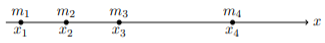
Example: Suppose we have two masses along the x-axis, mass  at position and mass
  at position
  . Where is the center of mass?
Answer: Intuitively we know that the center of mass is closer to the larger mass.
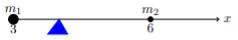
From physics, we know the center of mass is

We call this formula a “weighted” average of the  and
and  . Here is weighted more heavily because it has more mass.
Now look at the definition of expected value E(X). It is a weighted average of the values of X with the weights being probabilities  rather than masses! We might say that “The expected value is the point at which the distribution would balance.” Note the similarity between the physics example and the previous dice example.
Check Your Understanding: Mean of a Discrete Random Variable
Variance and Standard Deviation for Discrete Random Variables
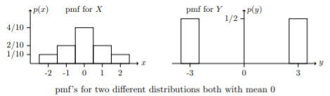
The expected value (mean) of a random variable is a measure of location or central tendency. If you had to summarize a random variable with a single number, the mean would be a desirable choice. Still, the mean leaves out a good deal of information. For example, the random variables X and Y below both have mean 0, but their probability mass is spread out about the mean quite differently.

It is probably a little easier to see the different spreads in plots of the probability mass functions. We use bars instead of dots to give a better sense of the mass.
Variance and Standard Deviation
Taking the mean as the center of a random variable’s probability distribution, the variance is a measure of how much the probability mass is spread out around this center.
Definition: If X is a random variable with mean  , then the variance of X is defined by

The standard deviation  of X is defined by

If the relevant random variable is clear from context, then the variance and standard deviation are often denoted by  and (“sigma”), just as the mean is (“mu”).
What does this mean? First, let us rewrite the definition explicitly as a sum. If X takes values with probability mass function, then
 .
.
In words, the formula for Var(X) says to take a weighted average of the squared distance to the mean. By squaring, we make sure we are averaging only non-negative values, so that the spread to the right of the mean will not cancel that to the left.
Note on units:
-
-
- has the same units as
- Var(X) has the same units as the square of X. So, if X is in meters, then Var(X) is in meters squared.
-
Because and X have the same units, the standard deviation is a natural measure of spread.
Variance and Standard Deviation of a Discrete Random Variable
Check Your Understanding: Variance and Standard Deviation for Discrete Random Variables
Bernoulli
Bernoulli Distributions
Model: The Bernoulli distribution models one trial in an experiment that can result in either a success or failure. This is the most important distribution and is also the simplest. A random variable X has a Bernoulli distribution with parameter p if:
-
-
- X takes the values 0 and 1.
 and
and 
-
We will write X ~ Bernoulli (p) or Ber (p), which is read “X follows a Bernoulli distribution with parameter ” or “ is drawn from a Bernoulli distribution with parameter p.”
A simple model for the Bernoulli distribution is to flip a coin with probability p of heads, with X = 1 on heads and X = 0 on tails. The general terminology is to say X is 1 on success and 0 on failure, with success and failure defined by the context.
Many decisions can be modeled as a binary choice, such as votes for or against a proposal. If p is the proportion of the voting population that favors the proposal, then the vote of a random individual is modeled by a Bernoulli (p).
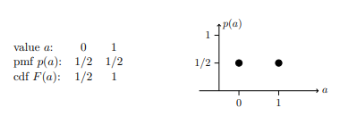
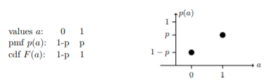
Here are the table and graphs of the pmf for the Bernoulli (1/2) distribution and below that for the general Bernoulli (p) distribution.
Mean and Variance of Bernoulli Distribution
Bernoulli Distribution Mean and Variance
The Variance of a Bernoulli Random Variable
Bernoulli random variables are fundamental, so we should know their variance.
If X~Bernoulli(p) then0

Proof: We know that E(X) = p. We compute Var(X) using a table (Table 4).
| values X | 0 | 1 |
|---|---|---|
| pmf p(x) | 1 – p | p |
| (X – )2 |
(0 – p)2 | (1 – p)2 |

Binomial Distributions
Binomial Variables
Check Your Understanding: Binomial Variables
Binomial Distribution
Visualizing a Binomial Distribution
Binomial Distributions
The binomial distribution Binomial (n,p), or Bin (n,p), models the number of successes in n independent Bernoulli(p) trials.
There is a hierarchy here. A single Bernoulli trial is, say, a toss of a coin. A single binomial trial consists of n Bernoulli trials. For coin flips the sample space for a Bernoulli trial is  . The sample space for a binomial trial is all sequences of heads and tails of length n. Likewise, a Bernoulli random variable takes values 0 and 1 and a binomial random variable takes values 0, 1, 2, …, n.
Example: The number of heads in n flips of a coin with probability p of heads follows a Binomial(n,p) distribution.
We describe X~Binomial(n,p) by giving its values and probabilities. For notation we will use k to mean an arbitrary number between 0 and n.
We remind you that ‘n choose k’  is the number of ways to choose k things out of a collection of n things and it has the formula

(It is also called a binomial coefficient). Table 5 is a table for the pmf of a Binomial(n,k) random variable:
| values a: | 0 | 1 | 2 | . . . | k | . . . | n |
|---|---|---|---|---|---|---|---|
| pmf p(a): |  |
 |
 |
. . . |  |
. . . | pn |
Example: What is the probability of 3 or more heads in 5 tosses of a fair coin?
Answer: The binomial coefficients associated with n = 5 are
 ,
, 
And similarly

Using these values, we get Table 6 for X~Binomial(5,p).
| values a: | 0 | 1 | 2 | 3 | 4 | 5 |
|---|---|---|---|---|---|---|
| pmf p(a): |  |
 |
 |
 |
 |
p5 |
We were told p = 1/2 so

Binomial Probability Example
Explanation of the Binomial Probabilities
For concreteness, let n = 5 and k = 2 (the argument for arbitrary n and k is identical). So X~Binomial(5,p) and we want to compute p(2). The long way to compute p(2) is to list all the ways to get exactly 2 heads in 5-coin flips and add up their probabilities. The list has 10 entries: HHTTT, HTHTT, HTTHT, HTTTH, THHTT, THTHT, THTTH, TTHHT, TTHTH, TTTHH.
Each entry has the same probability of occurring, namely

This is because each of the two heads has probability p and each of the 3 tails has probability 1 – p. Because the individual tosses are independent, we can multiply probabilities. Therefore, the total probability of exactly 2 heads is the sum of 10 identical probabilities, i.e.,  , as shown in Table 6.
This guides us to the shorter way to do the computation. We have to count the number of sequences with exactly 2 heads. To do this we need to choose 2 of the tosses to be heads and the remaining 3 to be tails. The number of such sequences is the number of ways to choose 2 out of the 5 things, which is  . Since each such sequence has the same probability,, we get the probability of exactly 2 heads
  .
.
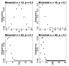
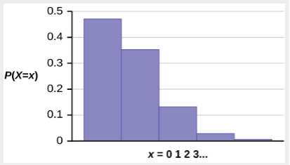
Here are some binomial probability mass functions (here, frequency is the same as probability).
Check Your Understanding: Binomial Probability
Characteristics of a Binomial Experiment
-
-
- There are a fixed number of trials. Think of trials as repetitions of an experiment. The letter n denotes the number of trials.
- The random variable, x, number of successes, is discrete.
- There are only two possible outcomes, called “success” and “failure,” for each trial. The letter p denotes the probability of a success on any one trial, and q denotes the probability of a failure on any one trial. p + q = 1
- The n trials are independent and are repeated using identical conditions. Think of this as drawing WITH replacement. Because the n trials are independent, the outcome of one trial does not help in predicting the outcome of another trial. Another way of saying this is that for each individual trial, the probability, p, of a success and probability, q, of a failure remain the same. For example, randomly guessing at a true-false statistics question has only two outcomes. If a success is guessing correctly, then a failure is guessing incorrectly. Suppose Jow always guesses correctly on any statistics true-false question with a probability
 . Then,
  . This means that for every true-false statistics question Joe answers, his probability of success () and his probability of failure () remain the same.
-
Any experiment that has characteristics three and four and where n = 1 is called the Bernoulli Trial.
A word about independence
So far, we have been using the notion of an independent random variable without ever carefully defining it. For example, a binomial distribution is the sum of independent Bernoulli trials. This may (should?) have bothered you. Of course, we have an intuitive sense of what independence means for experimental trials. We also have the probabilistic sense that random variables X and Y are independent if knowing the value of X gives you no information about the value of Y.
Definition: The discrete random variables X and Y are independent if

For any values a,b. That is, the probabilities multiply.
Expected Value of a Binomial Variable
Variance of a Binomial Variable
Finding the Mean and Standard Deviation of a Binomial Random Variable
Variance of Binomial (n,p)
Suppose X~Binomial(n,p). Since X is the sum of independent Bernoulli(p) variables and each Bernoulli variable has variance  we have

Check Your Understanding: Expected Value of a Binomial Variable
Geometric Distributions
Geometric Random Variables Introduction
Check Your Understanding: Binomial vs. Geometric Random Variables
Geometric Distributions
A geometric distribution models the number of tails before the first head in a sequence of coin flips (Bernoulli trials).
Example: (a) Flip a coin repeatedly. Let X be the number of tails before the first heads. So, X can equal 0, i.e., the first flip is heads, 1, 2, …. In principle, it takes any nonnegative integer value.
(b) Give a flip of tails the value 0 and heads the value 1. In this case, X is the number of 0’s before the first 1.
(c) Give a flip of tails the value 1 and heads the value 0. In this case, X is the number of 1’s before the first 0.
(d) Call a flip of tails a success and heads a failure. So, X is the number of successes before the first failure.
(e) Call a flip of tails a failure and heads a success. So, X is the number of failures before the first success.
You can see this models many different scenarios of this type. The most neutral language is the number of tails before the first head.
Formal definition: The random variable X follows a geometric distribution with parameter p if
- X takes the values 0, 1, 2, 3, …
- Its pmf is given by

We denote this by  . In Table 7 we have:
Unchanged:
| value | a: | a: | 0 | 1 | 2 | 3 | . . . | k | . . . |
|---|---|---|---|---|---|---|---|---|---|
| pmf | p(a): | p |  |
 |
 |
. . . |  |
. . . |

The geometric distribution is an example of a discrete distribution that takes an infinite number of possible values. Things can get confusing when we work with successes and failures since we might want to model the number of successes before the first failure, or we might want the number of failures before the first success. To keep things straight you can translate to the neutral language of the number of tails before the first heads.
Probability for a Geometric Random Variable
Characteristics of a Geometric Experiment
The geometric probability density function builds upon what we have learned from the binomial distribution. In this case, the experiment continues until either a success or a failure occurs rather than for a set number of trials. Here are the main characteristics of a geometric experiment:
-
-
-
- There are one or more Bernoulli trials with all failures except the last one, which is a success. In other words, you keep repeating what you are doing until the first success. Then you stop. For example, you throw a dart at a bullseye until you hit the bullseye. The first time you hit the bullseye is a “success,” so you stop throwing the dart. It might take six tries until you hit the bullseye. You can think of the trials as failure, failure, failure, failure, failure, success, STOP.
- In theory, the number of trials could go on forever.
- The probability, p, of a success and the probability, q, of a failure is the same for each trial. p + q = 1 and
 . For example, the probability of rolling a three when you throw one fair die is
  . This is true no matter how many times you roll the die. Suppose you want to know the probability of getting the first three on the fifth roll. On rolls one through four, you do not get a face with a three. The probability for each of the rolls is
  , the probability of a failure. The probability of getting a three on the fifth roll is
- X = the number of independent trials until the first success.
-
-
Check Your Understanding: Probability for a Geometric Random Variable
Cumulative Geometric Probability (greater than a value)
Cumulative Geometric Probability (less than a value)
Check Your Understanding: Cumulative Geometric Probability
Poisson Distributions
Poisson Process 1
Poisson Process 2
Poisson Distribution
Another useful probability distribution is the Poisson distribution or waiting time distribution. This distribution is used to determine how many checkout clerks are needed to keep the waiting time in line to specified levels, how many telephone lines are needed to keep the system from overloading, and many other practical applications. The distribution gets its name from Simeon Poisson who presented it in 1837 as an extension of the binomial distribution.
Here are the main characteristics of a Poisson experiment:
-
-
- The Poisson probability distribution gives the probability of a number of events occurring in a fixed interval of time or space if these events happen with a known average rate.
- The events are independent of the time since the last event. For example, a book editor might be interested in the number of words spelled incorrectly in a particular book. It might be that, on the average, there are five words spelled incorrectly in 100 pages. The interval is the 100 pages, and it is assumed that there is no relationship between when misspellings occur.
- The random variable X = the number of occurrences in the interval of interest.
-
Example: You notice that a news reporter says “uh,” on average, two times per broadcast. What is the probability that the news reporter says “uh” more than two times per broadcast?
This is a Poisson problem because you are interested in knowing the number of times the news reporter says “uh” during a broadcast.
(a) What is the interval of interest?
a. one broadcast measured in minutes
(b) What is the average number of times the news reporter says “uh” during one broadcast?
a. 2
(c) Let X = ____. What values does X take on?
a. Let X = the number of times the news reporter says “uh” during one broadcast. 
d. The probability question is P(__).
a. 
Notation for the Poisson: P = Poisson Probability Distribution Function

Read this as “X is a random variable with a Poisson distribution.” The parameter is  the mean for the interval of interest. The mean is the number of occurrences that occur on average during the interval period.
The formula for computing probabilities that are from a Poisson process is:

where P(X) is the probability of X successes, is the expected number of successes based upon historical data, e is the natural logarithm approximately equal to 2.718, and X is the number of successes per unit, usually per unit of time.
In order to use the Poisson distribution, certain assumptions must hold. These are: the probability of a success, , is unchanged within the interval, there cannot be simultaneous successes within the interval, and finally, that the probability of a success among intervals is independent, the same assumption of the binomial distribution.
In a way, the Poisson distribution can be thought of as a clever way to convert a continuous random variable, usually time, into a discrete random variable by breaking up time into discrete independent intervals. This way of thinking about the Poisson helps us understand why it can be used to estimate the probability for the discrete random variable from the binomial distribution. The Poisson is asking for the probability of a number of successes during a period of time while the binomial is asking for the probability of a certain number of successes for a given number of trials.
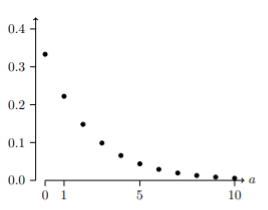
Example: Leah’s answering machine receives about six telephone calls between 8 a.m. and 10 a.m. What is the probability that Leah receives more than one call in the next 15 minutes?
Let X = the number of calls Leah receives in 15 minutes (the interval of interest is 15 minutes or  hour)
hour)
If Leah receives, on average, six telephone calls in two hours, and there are eight 15 minutes intervals in two hours, then Leah receives  calls in 15 minutes, on average. So,
  for this problem.


Probability that Leah receives more than one telephone call in the next 15 minutes is about 0.1734.
The graph of is:
The y-axis contains the probability of x where X = the number of calls in 15 minutes.
Poisson Probability Distribution – Example
Check Your Understanding: Poisson Distributions
Tables of Distributions and Properties
| Distribution | Range | pmf | Mean | Variance |
|---|---|---|---|---|
| Bernoulli(p) | 0,1 |  |
p | |
| Binomial(n,p) | 0, 1, … , n |  |
np |  |
| Geometric(p) | 0, 1, 2, … |  |
 |
 |
Let X be a discrete random variable with range 
| Expected Value: | Variance: |
|---|---|
| Synonyms: mean, average | |
Notation:  |
 |
Definition:  |
 |
Set Up and Work with Distributions for Continuous Random Variables
This section will explain how to work with distributions for continuous random variables. It will start with some definition and a calculus warm-up to help prepare you. The videos help explain the concepts while there are problems after each short section to help check your understanding.
Continuous Random Variables
We now turn to continuous random variables. All random variables assign a number to each outcome in a sample space. Whereas discrete random variables take on a discrete set of possible values, continuous random variables have a continuous set of values.
Computationally, to go from discrete to continuous we simply replace sums by integrals. It will help you to keep in mind that (informally) an integral is just a continuous sum.
Calculus Warmup
Conceptually, you should be comfortable with two views of a definite integral.


The connection between the two is seen below in Figure 11:

As the width  of the intervals gets smaller the approximation becomes better.
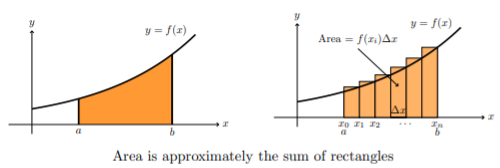
Note: In calculus, you learned to compute integrals by finding antiderivatives. This is important for calculations, but do not confuse this method for the reason we use integrals. Our interest in integrals comes primarily from its interpretation as a “sum” and to a much lesser extent its interpretation as area.
Probability Density Functions
Continuous Random Variables and Probability Density Functions
A continuous random variable takes a range of values, which may be finite in extent. Here are a few examples of ranges: ![[0,1],[0, \infty),(-\infty, \infty),[a, b] .](https://uta.pressbooks.pub/app/uploads/quicklatex/quicklatex.com-73a80af017dc82f40684a8c0003a4ff2_l3.png "Rendered by QuickLaTeX.com")
Definition: A random variable X is continuous if there is a function f (x) such that for any  we have

The function f (x) is called the probability density function (pdf).
The pdf always satisfies the following properties:
-
-
 (f is nonnegative).
 (This is equivalent to:
-
The probability density function f (x) of a continuous random variable is the analogue of the probability mass function p (x) of a discrete random variable. Here are two significant differences:
-
-
- Unlike p (x), the pdf f (x) is not a probability. You have to integrate it to get probability.
- Since f (x) is not a probability, there is no restriction that f (x) be less than or equal to 1.
-
Note: In property 2, we integrated over  since we did not know the range of values taken by X. Formally, this makes sense because we just define f (x) to be 0 outside of the range of X. In practice, we would integrate between bounds given by the range of X.
The Terms “Probability Mass” and “Probability Density”
Why do we use the terms mass and density to describe the pmf and pdf? What is the difference between the two? The simple answer is that these terms are completely analogous to the mass and density you saw in physics and calculus. We will review this first for the probability mass function and then discuss the probability density function. in extent.
Mass as a sum:
If masses  and are set in a row at positions
  , then the total mass is
We can define a ‘mass function’ p (x) with  for
for  and
and  otherwise. In this notation the total mass is

The probability mass function behaves in exactly the same way, except it has the dimension of probability instead of mass.
Mass as an integral of density:
Suppose you have a rod of length L meters with varying density f (x) kg/m. (Note the units are mass/length).
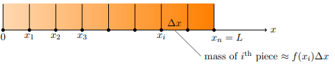
If the density varies continuously, we must find the total mass of the rod by integration: total mass =  .
.
This formula comes from dividing the rod into small pieces and ‘summing’ up the mass of each piece. That is: 
In the limit as goes to zero the sum becomes the integral.
The probability density function behaves exactly the same way, except it has units of probability/ (unit x) instead of kg/m. Indeed, the equation is exactly analogous to the above integral for total mass.
While we are on a physics kick, note that for both discrete and continuous random variables, the expected value is simply the center of mass or balance point.
Properties of Continuous Probability Density Functions
The graph of a continuous probability distribution is a curve. Probability is represented by area under the curve. The curve is called the probability density function (pdf). We use the symbol f (x) to represent the curve. f (x) is the function that corresponds to the graph; we use the density function f (x) to draw the graph of the probability distribution.
Area under the curve is given by a different function called the cumulative distribution function (cdf). The cumulative distribution function is used to evaluate probability as area. Mathematically, the cumulative probability density function is the integral of the pdf, and the probability between two values of a continuous random variable will be the integral of the pdf between these two values: the area under the curve between these values. Remember that the area under the pdf for all possible values of the random variable is one, certainty. Probability thus can be seen as the relative percent of certainty between the two values of interest.
- The outcomes are measured, not counted.
- The entire area under the curve and above the x-axis is equal to one.
- Probability is found for intervals of x values rather than for individual x values.
 is the probability that the random variable X is in the interval between the values c and d. is the area under the curve, above the x-axis, to the right of c and the left of d.
 The probability that x takes on any single individual value is zero. The area below the curve, above the x-axis, and between x = c and x = c has no width, and therefore no area (area= 0). Since the probability is equal to the area, the probability is also zero.
 is the same as
  because probability is equal to area.
We will find the area that represents probability by using geometry, formulas, technology, or probability tables. In general, integral calculus is needed to find the area under the curve for many probability density functions.
There are many continuous probability distributions. When using a continuous probability distribution to model probability, the distribution used is selected to model and fit the particular situation in the best way.
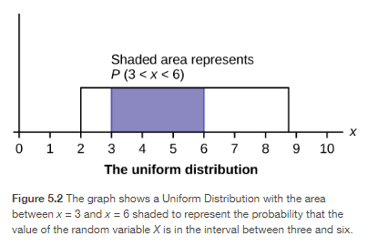
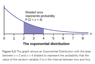
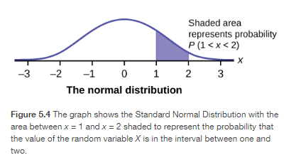
In this section, we will study the uniform distribution, the exponential distribution, and the normal distribution. The following graphs illustrate these distributions.
Cumulative Distribution Function
The cumulative distribution function (cdf) of a continuous random variable X is defined in exactly the same way as the cdf of a discrete random variable.

Note well that the definition is about probability. When using the cdf you should first think of it as a probability. Then when you go to calculate it, you can use

Notes:
-
-
- For discrete random variables, there was not much occasion to use the cumulative distribution function. The cdf plays a far more prominent role for continuous random variables.
- As before, we started the integral at
 because we did not know the precise range of X. Formally, this still makes sense since
  outside the range of X. In practice, we will know the range and start the integral at the start of the range.
 - In practice, we often say “X has distribution F (x)” rather than “X has cumulative distribution function F (x).”
-
Check Your Understanding: Continuous Random Variables
Uniform Distributions
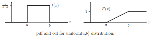
The Uniform Distribution
The uniform distribution is a continuous probability distribution and is concerned with events that are equally likely to occur. When working out problems that have a uniform distribution, be careful to not if the data is inclusive or exclusive of endpoints.
The mathematical statement of the uniform distribution is

Where a = the lowest value of x and b = the highest value of x.
Formulas for the theoretical mean and standard deviation are

Uniform Distribution Properties
-
-
- Parameters: a, b
- Range: [a, b]
- Notation: uniform

- Density:
- Distribution:

- Models: All outcomes in the range have equal probability (more precisely all outcomes have the same probability density).
-
Graphs:
Examples:
-
-
- Suppose we have a tape measure with markings at each millimeter. If we measure (to the nearest marking) the length of items that are roughly a meter long, the rounding error will uniformly distributed between

- Many boardgames use spinning arrows (spinners) to introduce randomness. When spun, the arrow stops at an angle that is uniformly distributed between 0 and
 radians.
 - In most pseudo-random number generators, the basic generator simulates a uniform distribution, and all other distributions are constructed by transforming the basic generator.
- Suppose we have a tape measure with markings at each millimeter. If we measure (to the nearest marking) the length of items that are roughly a meter long, the rounding error will uniformly distributed between
-
Check Your Understanding: Uniform Distributions
Exponential Distributions
The Exponential Distribution
The exponential distribution is often concerned with the amount of time until some specific occurs. For example, the amount of time (beginning now) until an earthquake occurs has an exponential distribution. Other examples include the length of time, in minutes, of long-distance business telephone calls, and the amount of time, in months, a car battery lasts. It can be shown, too, that the value of the change that you have in your pocket or purse approximately follows an exponential distribution.
Values for an exponential random variable occur in the following way. There are fewer large values and more small values. For example, marketing studies have shown that the amount of money customers spend in one trip to the supermarket follows an exponential distribution. There are more people who spend small amounts of money and fewer people who spend large amounts of money.
Exponential distributions are commonly used in calculations of product reliability, or length of time a produce lasts.
The random variable for the exponential distribution is continuous and often measures a passage of time, although it can be used in other applications. Typical questions may be, “what is the probability that some event will occur within the next x hours or days, or what is the probability that some event will occur between  hours, or what is the probability that the event will take more than hours to perform?” In short, the random variable X equals (a) the time between events or (b) the passage of time to complete an action, e.g., wait on a customer. The probability density function is given by:

Where is the historical average waiting time and has a mean and standard deviation of  .
.
In order to calculate probabilities for specific probability density functions, the cumulative density function is used. The cumulative density function (cdf) is simply the integral of the pdf and is:
![F(x)=\int_0^{\infty}\left[\frac{1}{\mu} e^{-\frac{x}{\mu}}\right]=1-e^{-\frac{x}{\mu}}](https://uta.pressbooks.pub/app/uploads/quicklatex/quicklatex.com-8c7318082a78c2222cd0e9b1bf519d28_l3.png "Rendered by QuickLaTeX.com")
Example
Check Your Understanding: Exponential Probability Distribution
Integration by Parts – Exponential Distribution
Memorylessness of the Exponential Distribution
Say that the amount of time between customers for a postal clerk is exponentially distributed with a mean of two minutes. Suppose that five minutes have elapsed since the last customer arrived. Since an unusually long amount of time has now elapsed, it would seem to be more likely for a customer to arrive within the next minute. With the exponential distribution, this is not the case – the additional time spend waiting for the next customer does not depend on how much time has already elapsed since the last customer. This is referred to as the memoryless property. The exponential and geometric probability density functions are the only probability functions that have the memorylessmemoryless property. property. Specifically, the memoryless property says that

For example, if five minutes have elapsed since the last customer arrives, then the probability that more than one minute will elapse before the next customer arrives is computed by using  in the foregoing equation.

This is the same probability as tat of waiting more than one minute for a customer to arrive after the previous arrival.
Check Your Understanding: Memorylessness of the Exponential Distribution
Relationship Between the Poisson and the Exponential Distribution
There is an interesting relationship between the exponential distribution and the Poisson distribution. Suppose that the time that elapses between two successive events follows the exponential distribution with a mean of units of time. Also assume that these times are independent, meaning that the time between events is not affected by the times between previous events. If these assumptions hold, then the number of events per unit of time follows a Poisson distribution with mean . Recall that if X has the Poisson distribution with mean , then

The formula for the exponential distribution:  . Where
  average time between occurrences.
We see that the exponential is the cousin of the Poisson distribution, and they are linked through this formula. There are important differences that make each distribution relevant for different types of probability problems.
First, the Poisson has a discrete random variable, x =, where time; a continuous variable is artificially broken into discrete pieces. We saw that the number of occurrences of an event in a given time interval, x, follows the Poisson distribution.
For example, the number of times the telephone rings per hour. By contrast, the time between occurrences follows the exponential distribution. For example, the telephone just rang, how long will it be until it rings again? We are measuring length of time of the interval, a continuous random variable, exponential, not events during an interval, Poisson.
The Exponential Distribution v. the Poisson Distribution
A visual way to show both the similarities and differences between these two distributions is with a timeline.
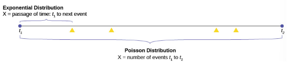
The random variable for the Poisson distribution is discrete and thus counts events during a given time period,  on Figure 19 above and calculates the probability of that number occurring. The number of events, four in the graph is measured in counting numbers; therefore, the random variable of the Poisson is a discrete random variable.
The exponential probability distribution calculates probabilities of the passage of time, a continuous random variable. In Figure 19, this is shown as the bracket from  to the next occurrence of the event marked with a triangle.
Classic Poisson distribution questions are “how many people will arrive at my checkout window in the next hour?”
Classic exponential distribution questions are “how long it will be until the next person arrives,” or a variant, “how long will the person remain here once they have arrived?”
Again, the formula for the exponential distribution is:

We see immediately the similarity between the exponential formula and the Poisson formula.
Both probability density functions are based upon the relationship between time and exponential growth or decay. The “e” in the formula is a constant with the approximate value of 2.71828 and is the base of the natural logarithmic exponential growth formula. When people say that something has grown exponentially this is what they are talking about.
An example of the exponential and the Poisson will make clear the differences been the two. It will also show the interesting applications they have.
Poisson Distribution
Suppose that historically 10 customers arrive at the checkout lines each hour. Remember that this is still probability, so we have to be told these historical values. We see this is a Poisson probability problem.
We can put this information into the Poisson probability density function and get a general formula that will calculate the probability of any specific number of customers arriving in the next hour.
The formula is for any value of the random variable we chose, and so the x is put into the formula. This is the formula:

As an example, the probability of 15 people arriving at the checkout counter in the next hour would be

Here we have inserted x = 15 and calculated the probability that in the next hour 15 people will arrive is .061.
Exponential Distribution
If we keep the same historical facts that 10 customers arrive each hour, but we now are interested in the service time a person spends at the counter, then we would use the exponential distribution. The exponential probability function for any value of x, the random variable, for this particular checkout counter historical data is:

To calculate , the historical average service time, we simply divide the number of people that arrive per hour, 10, into the time period, one hour, and have  . Historically, people spend 0.1 of an hour at the checkout counter, or 6 minutes. This explains the .1 in the formula.
There is a natural confusion with in both the Poisson and exponential formulas. They have different meanings, although they have the same symbol. The mean of the exponential is one divided by the mean of the Poisson. If you are given the historical number of arrivals, you have the mean of the Poisson. If you are given an historical length of time between events, you have the mean of an exponential.
Continuing with our example at the checkout clerk; if we wanted to know the probability that a person would spend 9 minutes or less checking out, then we use this formula. First, we convert to the same time units which are parts of one hour. Nine minutes is 0.15 of one hour. Next, we note that we are asking for a range of values. This is always the case for a continuous random variable. We write the probability question as:

We can now put the numbers into the formula, and we have our result

The probability that a customer will spend 9 minutes or less checking out is 0.7769.
We see that we have a high probability of getting out in less than nine minutes and a tiny probability of having 15 customers arriving in the next hour.
Exponential Distribution Properties
-
-
- Parameter:

- Range:

- Notation: exponential

- Density:

- Distribution: (easy integral)

- Right tail distribution:

- Models: The waiting time for a continuous process to change state.
- Parameter:
-
Examples:
-
-
- If I step out to 77 Mass Ave after class and wait for the next taxi, m waiting time in minutes is exponentially distributed. We will see that in this case
 is given by one over the average number of taxis that pass per minute (on weekday afternoons).
 - The exponential distribution models the waiting time until an unstable isotope undergoes nuclear decay. In this case, the value of is related to the half-life of the isotope.
- If I step out to 77 Mass Ave after class and wait for the next taxi, m waiting time in minutes is exponentially distributed. We will see that in this case
-
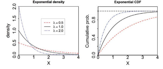
Graphs:
The Normal Distribution
The normal probability density function, a continuous distribution, is the most important of all the distributions. It is widely used and even more widely abused. Its graph is bell-shaped. You see the bell curve in almost all disciplines. Some of these include psychology, business, economics, the sciences, nursing, and, of course, mathematics. Some of your instructors may use the normal distribution to help determine your grade. Most IQ scores are normally distributed. Often real-estate prices fit a normal distribution.
The normal distribution has two parameters (two numerical descriptive measures): the mean  and the standard deviation
  . If X is a quantity to be measured that has a normal distribution with mean and standard deviation , we designate this by writing the following formula of the normal probability density function:
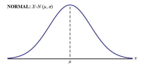
The probability density function is a rather complicated function. Do not memorize it. It is not necessary.

The curve is symmetric about a vertical line drawn through the mean,  The mean is the same as the median, which is the same as the mode, because the graph is symmetric about As the notation indicates, the normal distribution depends only on the mean and the standard deviation. Note that this is unlike several probability density functions we have already studies, such as the Poisson, where the mean is equal to
  and the standard deviation simply the square root of the mean, or the binomial, where p is used to determine both the mean and standard deviation. Since the area under the curve must equal one, a change in the standard deviation, , causes a change in the shape of the normal curve; the curve becomes fatter and wider or skinnier and taller depending on . A change in causes the graph to shift to the left or right. This means there are an infinite number of normal probability distributions. One of the special interests is called the standard normal distribution.
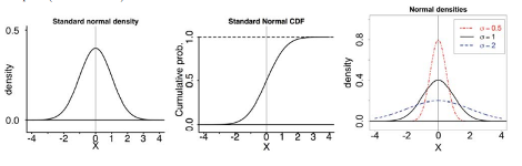
The Standard Normal Distribution
The standard normal distribution is a normal distribution of standardized values called z—scores. A z-score is measure in units of the standard deviation.
The mean for the standard normal distribution is zero, and the standard deviation is one. What this does is dramatically simplify the mathematical calculation of probabilities. Take a moment and substitute zero and one in the appropriate places in the above formula and you can see that the equation collapses into one that can be much more easily solved using integral calculus. The transformation  produces the distribution
  . The value x in the given equation comes from a known normal distribution with known mean and known standard deviation . The z-score tells how many standard deviations a particular x is away from the mean.
Z-Scores
If X is a normally distributed random variable and  , then the z-score for a particular x is:
The z-score tells you how many standard deviations the value x is above (to the right of) or below (to the left of) the mean,  . Values of x that are larger than the mean have positive z-scores, and values of x that are smaller than the mean have negative z-scores. If x equals the mean, then x has a z-score of zero.
Example: Suppose  . This says that X is a normally distributed random variable with mean
  and standard deviation
  . Suppose
  . Then:

This means that is two standard deviations  above or to the right of the mean .
Now suppose x = 1. Then:  (rounded to two decimal places).
This means that x = 1 is 0.67 standard deviations  below or to the left of the mean .
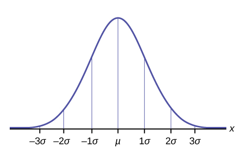
The Empirical Rule
If X is a random variable and has a normal distribution with mean and standard deviation , then the Empirical Rule states the following:
- About 68% of the x values lie between
 of the mean (within one standard deviation of the mean).
 - About 95% of the x values lie between
 (within two standard deviations of the mean).
 - About 99.7% of the x values lie between
 of the mean (within three standard deviations of the mean). Notice that almost all the x values lie within three standard deviations of the mean.
 - The z-scores for
 respectively
 - The z-scores for
 respectively.
 - The z-scores for
 respectively.
Normal Distribution Problems: Empirical Rule
Check Your Understanding: Normal Distribution Problems
Normal Distribution Properties
In 1809, Carl Friedrich Gauss published a monograph introducing several notions that have become fundamental to statistics: the normal distribution, maximum likelihood estimation, and the method of least squares. For this reason, the normal distribution is also called the Gaussian distribution, and it is the most important continuous distribution.
-
-
- Parameters:

- Range:
- Notation: normal

- Density:

- Distribution:
 has no formula, so use tables or software such as “pnorm” in R to compute F(x). (Will be discussed later in the module)
 - Models: Measurement error, intelligence/ability, height, averages of lots of data.
- Parameters:
-
Here are some graphs of normal distributions. Note they are shaped like a bell curve. Note also that as increases as they become more spread out.
Using the Normal Distribution
The shaded area in Figure 24 indicates the area to the right of x. This area is represented by the probability  . Normal tables provide the probability between the mean, zero for the standard normal distribution, and a specific value such as . This is the unshaded part of the graph from the mean to .
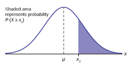
Because the normal distribution is symmetrical, if were the same distance to the left of the mean the area, probability, in the left tail, would be the same as the shaded area in the right tail. Also, bear in mind that because of the symmetry of this distribution, one-half of the probability is to the right of the mean and one-half is to the left of the mean.
Calculations of Probabilities
To find the probability for probability density functions with a continuous random variable we need to calculate the area under the function across the values of X we are interested in. For the normal distribution this seems a difficult task given the complexity of the formula. There is, however, a simple way to get what we want. Here again is the formula for the normal distribution:

Looking at the formula for the normal distribution it is not clear just how we are going to solve for the probability doing it the same way we did it with the previous probability functions. There we put the data into the formula and did the math.
To solve this puzzle, we start knowing that the area under a probability density function is the probability.
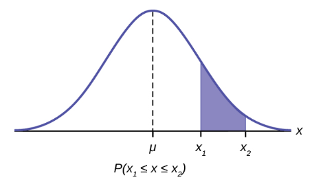
This shows that the area between  is the probability as stated in the formula:
The mathematical tool needed to find the area under a curve is integral calculus. The integral of the normal probability density function between the two points  is the area under the curve between these two points and is the probability between these two points.
Doing these integrals is no fun and can be very time consuming. But now, remembering that there are an infinite number of normal distributions out there, we can consider the one with a mean of zero and a standard deviation of 1. This particular normal distribution is given the name Standard Normal Distribution. Putting these values into the formula it reduces to a very simple equation. We can now quite easily calculate all probabilities for any value of x, for this particular normal distribution, that has a mean of zero and a standard deviation of 1. They are presented in numerous ways. The table is the most common presentation and is set up with probabilities for one-half the distribution beginning with zero, the mean, and moving outward. The shaded area in the graph at the top of the table in Statistical Tables represents the probability from zero to the specific Z value noted on the horizontal axis, Z.
The only problem is that even with this table, it would be a ridiculous coincidence that our data had a mean of zero and a standard deviation of one. The solution is to convert the distribution we have with its mean and standard deviation to this new Standard Normal Distribution. The Standard Normal has a random variable called Z.
Using the standard normal table, typically called the normal table, to find the probability of one standard deviation, go to the Z column, reading down to 1.0 and then read at column 0. That number, 0.3413 is the probability from zero to 1 standard deviation. At the top of the table is the shaded area in the distribution which is the probability for one standard deviation. The table has solved our integral calculus problem. But only if our data has a mean of zero and a standard deviation of 1.
However, the essential point here is, the probability for one standard deviation on one normal distribution is the same on every normal distribution. If the population data set has a mean of 10 and a standard deviation of 5 then the probability from 10 to 15, one standard deviation, is the same as from zero to 1, one standard deviation on the standard normal distribution. To compute probabilities, areas, for any normal distribution, we need only to convert the particular normal distribution to the standard normal distribution and look up the answer in the tables. As review, here again is the standardizing formula:

where Z is the value on the standard normal distribution, X is the value from a normal distribution one wishes to convert to the standard normal, μ and σ are, respectively, the mean and standard deviation of that population. Note that the equation uses μ and σ which denotes population parameters. This is still dealing with probability, so we always are dealing with the population, with known parameter values and a known distribution. It is also important to note that because the normal distribution is symmetrical it does not matter if the z-score is positive or negative when calculating a probability. One standard deviation to the left (negative Z-score) covers the same area as one standard deviation to the right (positive Z-score). This fact is why the Standard Normal tables do not provide areas for the left side of the distribution. Because of this symmetry, the Z-score formula is sometimes written as:

Where the vertical lines in the equation means the absolute value of the number. What the standardizing formula is really doing is computing the number of standard deviations X is from the mean of its own distribution.
Check Your Understanding: Using the Normal Distribution
Probabilities from Density Curves
Check Your Understanding: Probabilities from Density Curves
Standard Normal Table for Proportion Below
Standard Normal Table for Proportion Above
Check Your Understanding: Standard Normal Table for Proportion Below and Above
Standard Normal Table for Proportion Between Values
Check Your Understanding: Standard Normal Table for Proportion Between Values
Finding z-score for a Percentile
Check Your Understanding: Finding z-score for a Percentile
Expectation, Variance and Standard Deviation for Continuous Random Variables
So far, we have looked at expected value, standard deviation, and variance for discrete random variables. These summary statistics have the same meaning for continuous random variables:
- The expected value
 is a measure of location or central tendency.
 - The standard deviation is a measure of the spread or scale.
- The variance
 is the square of the standard deviation.
To move from discrete to continuous, we will simply replace the sums in the formulas by integrals.
Expected Value of a Continuous Random Variable
Definition: Let X be a continuous random variable with range ![[a, b]](https://uta.pressbooks.pub/app/uploads/quicklatex/quicklatex.com-b28ebca9266518f1a778b4a4b102a2e1_l3.png "Rendered by QuickLaTeX.com") and probability density function
and probability density function  . The expected value of X is defined by

Let us see how this compares with the formula for a discrete random variable:

The discrete formula says to take a weighted sum of the values  , where the weights are the probabilities . Recall that is a probability density. Its units are prob/(unit of X).
So,  represents the probability that X is in an infinitesimal range of width dx around x. Thus, we can interpret the formula for E(X) as a weighted integral of the values x of X, where the weights are the probabilities f(x)dx.
As before, the expected value is also called the mean or average.
Example 1: Let  .
.
Answer: X has range [0,1] and density  . Therefore,

Not surprisingly the mean is at the midpoint of the range.
Example 2: Let X have a range ![[0,2] \text { and density } \frac{3}{8} x^2 \text {. Find } E(X) \text {. }](https://uta.pressbooks.pub/app/uploads/quicklatex/quicklatex.com-3bc58e73bd8c109b288d9bd49e61cdd5_l3.png "Rendered by QuickLaTeX.com") .
.
Answer: 
Does it make sense that this X has mean in the right half of its range?
Yes. Since the probability density increases as x increases over the range, the average value of x should be in the right half of the range.
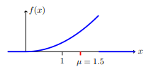
is “pulled” to the right of the midpoint 1 because there is more mass to the right.
Example 3: Let  .
.
Answer: The range of  .
.

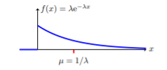
Example 4: Let  .
.
Answer: The range of 

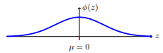
Properties of E(X)
The properties of E(X) for continuous random variables are the same as for discrete ones:
-
-
-
- If X and Y are random variables on a sample space,
 then
then 
- If a and b are constants, then

- If X and Y are random variables on a sample space,
-
-
Example 5: In this example we verify that for we have .
Answer: Example (4) showed that for standard normal Z,  . We could mimic the calculation there to show that . Instead, we will use the linearity properties of
  .
.  is a normal random variable we can standardize it:

Inverting this formula, we have  . The linearity of expected value now gives

Expectation of Functions of X
This works exactly the same as the discrete case. If  is a function, then
  is a random variable and

Example 6: Let 
Answer: Using integration by parts we have
![\begin{gathered} E\left(X^2\right)=\int_0^{\infty} x^2 \lambda e^{-\lambda x} d x=\left[-x^2 e^{-\lambda x}-\frac{2 x}{\lambda} e^{-\lambda x}-\frac{2}{\lambda^2} e^{-\lambda x}\right]_0^{\infty} \\ =\frac{2}{\lambda^2} \end{gathered}](https://uta.pressbooks.pub/app/uploads/quicklatex/quicklatex.com-e39e2e26922ea44a094e333a849f2fe0_l3.png "Rendered by QuickLaTeX.com")
Variance
Now that we have defined expectation for continuous random variable, the definition of variance is identical to that of discrete random variables.
Definition: Let X be a continuous random variable with mean . The variance of X is
Properties of Variance
These are exactly the same as in the discrete case.
-
-
-
- If X and Y are independent, then

- For constants a and b,
 .
. - Theorem:

- If X and Y are independent, then
-
-
For Property 1, note carefully the requirement that X and Y are independent.
Property 3 gives a formula for  that is often easier to use in hand calculations.
Example 7: Let 
Answer: In Example 1 we found  . Next, we compute

Example 8: Let 
Answer: In Examples 3 and 6 we computed

So, by Property 3,

We could have skipped Property 3 and computed this directly from

Example 9: Let 
Note: The notation for normal variables is . This is certainly suggestive, but as mathematicians we need to prove that  . Above we showed . This example shows that
  , just as the notation suggests. In the next example we will show
Answer: Since , we have

(Using integration by parts with 


The first term equals 0 because the exponential goes to zero much faster than z grows at both  . The second term equals 1 because it is exactly the total probability integral of the pdf
  .
.
Example 10: Let 
Answer: This is an exercise in change of variables. Letting  , we have

The integral in the last line is the same one we computed for  .
.
Quantiles
Definition: The median of X is the value x for which  , i.e. the value of x such that
  . In other words, X has equal probability of being above or below the median, and each probability is therefore ½. In terms of the cdf
  , we can equivalently define the median as the value x satisfying
  .
.
Think: What is the median of Z?
Answer: By symmetry, the median is 0.
Example 11: Find the median of  .
.
Answer: The cdf of  . So, the median is the value of x for which
  . Solving for x we find:
  .
.
Think: In this case the median does not equal the mean of  . Based on the graph of the pdf of X can you argue why the median is to the left of the mean.
Definition: The 
Notes:
-
-
- In this notation the median is

- We will usually write this in terms of the cdf:

- In this notation the median is
-
With respect to the pdf  is the value such that there is an area of p to the left of
  and an area of
  to the right of . In the examples below, note how we can represent the quartile graphically using either area of the pdf or height of the cdf.
Example 12: Find the 0.6 quantile for  .
.
Answer: The cdf for ![X \text { is } F(x)=x \text { on the range }[0,1] \text {. So } q_{0.6}=0.6](https://uta.pressbooks.pub/app/uploads/quicklatex/quicklatex.com-c6a4a16f7520d934734391d0187ebf01_l3.png "Rendered by QuickLaTeX.com")
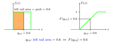
Quantile give a useful measure of location for a random variable.
Percentiles, decile, quartiles
For convenience, quantiles are often described in terms of percentile, decile, or quantiles. The 60th percentile is the same as the 0.6 quantile. For example, you are in the 60th percentile for height if you are taller than 60 percent of the population, i.e., the probability that you are taller than a randomly chosen person is 60 percent.
Likewise, deciles represent steps of 1/10. The third decile is the 0.3 quantile. Quartiles are in steps of ¼. Third quartile is the 0.75 quantile and the 75th percentile.
Relevance to Transportation Engineering Coursework
This section will relate the fundamentals of transportation engineering by discussion and showing you queuing theory and models to help your understanding.
Queuing Theory: Exponential Distribution
Poisson Model of Vehicle Arrivals
The Poisson distribution is used to represent arrival patterns at a roadway location to conduct traffic queue and delay analysis. The distribution helps estimate the likelihood of n vehicles arriving in a specific time frame and the average arrival rate using data collected from roadway locations. For more information on the Poisson distribution, the reader is referred to in the above section labeled “Poisson Distributions.”
Distribution of Time-Mean Speed
Spot speed studies during relatively congestion-free durations are conducted to estimate mean speed, modal speed, pace, standard deviation, and different percentile of speeds at a roadway location. 85th percentile speed estimated from a spot speed study is one of the crucial measures for determining the appropriate speed limit for the roadway section. Speed data for automobiles on roadway locations collected as part of the spot speed study typically follow the normal distribution discussed in “The Normal Distribution” section above.
Traffic Safety
Traffic safety analysis involves statistical methods that are used to process records of historical collisions or crash data. The negative binomial distribution is used to describe crash occurrences on roadway segments and intersections. The negative binomial model’s formulation is a variant of Poisson’s distribution (see “Poisson Distributions” above) that allows the standard deviation of the sample to exceed the mean.
Key Takeaways
- Probability distribution functions (PDFs) discussed in the chapter are used in several transportation engineering modeling applications. For example, arrival patterns at a roadway location critical to queue analysis follow a Poisson’s distribution while the time interval between arrivals follows a negative binomial distribution.
- Negative binomial distribution and its variants are also used to model collision frequency on road segments and intersections. These models, known as Safety Performance Functions, are used to estimate expected crash frequency on roadway entities.
- Data from spot speed studies are used to ensure that the roadway design context aligns with the posted speed limit. The speeds on the roadway segments with no congestion follow a normal distribution, and the data are used to estimate the mean, median, and 85th percentile of the normal distribution.
Glossary: Key Terms
Bayes’ Theorem[2] – a useful tool for calculating conditional probability. Bayes’Bernoulli trials. theorem can be expressed as: 𝐴1, 𝐴2,…, 𝐴𝑛 be a set of mutually exclusive events that together form the sample space S. Let B be any event from the same sample space, such that 𝑃(𝐵)>0. Then, 
Bernoulli Trials[1] – an experiment with the following characteristics: (1) There are only two possible outcomes called “success” and “failure” for each trial. (2) The probability p of a success is the same for any trial (so the probability 𝑞=1−𝑝 of a failure is the same for any trial).
Binomial Experiment[1] – a statistical experiment that satisfies the following three conditions: (1) There are a fixed number of trials, n. (2) There are only two possible outcomes, called “success” and, “failure,” for each trial. The letter p denotes the probability of a success on one trial, and q denotes, the probability of a failure on one trial. (3) The n trials are independent and are repeated using identical conditions.
Binomial Probability Distribution[1] – a discrete random variable that arises from Bernoulli trials; there are a fixed number, n, of independent trials. “Independent” means that the result of any trial (for example, trial one) does not affect the results of the following trials, and all trials are conducted under the same conditions. Under these circumstances the binomial random variable X is defined as the number of successes in n trials. The mean is 𝜇=𝑛𝑝 and the standard deviation is  The probability of exactly x successes in n trials is
Combination[2]– a combination is a selection of all or part of a set of objects, without regard to the order in which objects are selected
Conditional Probability[1] – the likelihood that an event will occur given that another event has already occurred.
Discrete Variable / continuous variable[2]– if a variable can take on any value between its minimum value and its maximum value, it is called a continuous variable; otherwise it is called a discrete variable
Expected Value[2] – the mean of the discrete random variable X is also called the expected value of X. Notationally, the expected value of X is denoted by 𝐸(𝑋).
Exponential Distribution[1] – a continuous random variable that appears when we are interested in the intervals of time between some random events, for example, the length of time between emergency arrivals at a hospital. The mean is  and the standard deviation is
  . The probability density function is
Geometric Distribution[1] – a discrete random variable that arises from the Bernoulli trials; the trials are repeated until the first success. The geometric variable X is defined as the number of trials until the first success. The mean is  The probability of exactly x failures before the first success is given by the formula: 𝑃(𝑋=𝑥)=𝑝(1−𝑝)𝑥−1 where one wants to know probability for the number of trials until the first success: the xth trial is the first success. An alternative formulation of the geometric distribution asks the question: what is the probability of x failures until the first success? In this formulation the trial that resulted in the first success is not counted. The formula for this presentation of the geometric is: 𝑃(𝑋=𝑥)=𝑝(1−𝑝)𝑥. The expected value in this form of the geometric distribution is
  . The easiest way to keep these two forms of the geometric distribution straight is to remember that p is the probability of success and (1−𝑝) is the probability of failure. In the formula the exponents simply count the number of successes and number of failures of the desired outcome of the experiment. Of course the sum of these two numbers must add to the number of trials in the experiment.
Geometric Experiment[1] – a statistical experiment with the following properties: (1) There are one or more Bernoulli trials with all failures except the last one, which is a success. (2) In theory, the number of trials could go on forever. There must be at least one trial. (3) The probability, p, of a success and the probability, q, of a failure do not change from trial to trial.
Independent[2] – two events are independent when the occurrence of one does not affect the probability of the occurrence of the other
Mean[2]– a mean score is an average score, often denoted by  . It is the sum of individual scores divided by the number of individuals.
Memoryless Property[1] – For an exponential random variable X, the memoryless property is the statement that knowledge of what has occurred in the past has no effect on future probabilities. This means that the probability that X exceeds 𝑥+𝑡, given that it has exceeded x, is the same as the probability that X would exceed t if we had no knowledge about it. In symbols we say that  .
.
Multiplication Rule[2] – If events A and B come from the same sample space, the probability that both A and B occur is equal to the probability the event A occurs time the probability that B occurs, given that A has occurred.  .
.
Normal Distribution[1] – a continuous random variable with pdf  , where 𝜇 is the mean of the distribution and 𝜎 is the standard deviation; notation:
  , the random variable, Z, is called the standard normal distribution
Permutation[2]– an arrangement of all or part of a set of objects, with regard to the order of the arrangement.
Poisson Distribution[1] – If there is a known average of 𝜇 events occurring per unit time, and these events are independent of each other, then the number of events X occurring in one unit of time has the Poisson distribution. The probability of x events occurring in one unit time is equal to
Poisson Probability Distribution[1] – a discrete random variable that counts the number of times a certain event will occur in a specific interval; characteristics of the variable: (1) the probability that the event occurs in a given interval is the same for all intervals. (2) the events occur with a known mean and independently of the time since the last event. The distribution is defined by the mean 𝜇 of the event in the interval. The mean is 𝜇=𝑛𝑝. The standard deviation is  . The probability of having exactly x successes in r trials is . The Poisson distribution is often used to approximate the binomial distribution, when n is “large” and p is “small” (a general rule is that np should be greater than or equal to 25 and p should be less than or equal to 0.01).
Probability Distribution Function (PDF)[1]– a mathematical description of a discrete random variable, given either in the form of an equation (formula) or in the form of a table listing all the possible outcomes of an experiment and the probability associated with each outcome.
Quartile[2] – Quartiles divide a rank-ordered data set into four equal parts. The values that divide each part are called the first, second, and third quartiles; and they are denoted by
Random Variable[1] – a characteristic of interest in a population being studied; common notation for variables are upper case Latin letters X, Y, Z..; common notation for a specific value from the domain (set of all possible values of a variable) are lower case Latin letters x, y, and z. For example, if X is the number of children in a family, then x represents a specific integer 0, 1, 2, 3,… Variables in statistics differ from variables in intermediate algebra in the two following ways: (1) The domain of the random variable is not necessarily a numerical set; the domain may be expressed in words; for example, if X = hair color then domain is {black, blonde, gray, green, orange}. (2) We can tell what specific value x the random variable X takes only after performing the experiment.
Standard Deviation[2] – The standard deviation is a numerical value used to indicate how widely individuals in a group vary. If individual observations vary greatly from the group mean, the standard deviation is big; and vice versa. It is important to distinguish between the standard deviation of a population and the standard deviation of a sample. They have different notation, and they are computed differently. The standard deviation of a population is denoted by 𝜎 and the standard deviation of a sample, by 𝑠
Standard Normal Distribution[1] – a continuous random variable 𝑋~𝑁(0,1); when X follows the standard normal distribution, it is often noted as 𝑍~𝑁(0,1).
Uniform Distribution[1] – a continuous random variable that has equally likely outcomes over the domain, 𝑎<𝑥<𝑏; it is often referred as the rectangular distribution because the graph of the pdf has the form of a rectangle. The mean is  and the standard deviation is
  The probability density function is
 ![f(x)=\frac{1}{b-a} \text { for } a<x. The cumulative distribution is [latex]P(X \leq x)=](https://uta.pressbooks.pub/app/uploads/quicklatex/quicklatex.com-91a16945b904adb5e47be9b5f750cafd_l3.png "Rendered by QuickLaTeX.com")

Variance[2] – the variance is a numerical value used to indicate how widely individuals in a group vary. If individual observations vary greatly from the group mean, the variance is big; and vice versa. It is important to distinguish between the variance of a population and the variance of a sample. They have different notation, and they are computed differently. The variance of a population is denoted by 𝜎2; and the variance of a sample, by 𝑠2
Z-Score[1] – the linear transformation of the form  ; if this transformation is applied to any normal distribution 𝑋~𝑁(𝜇,𝜎) the result is the standard normal distribution 𝑍~𝑁(0,1). If this transformation is applied to any specific value x of the random variable with mean 𝜇 and standard deviation 𝜎, the result is called the z-score of x. The z-score allows us to compare data that are normally distributed but scaled differently. A z-score is the number of standard deviations a particular x is away from its mean value.
[1] “Introductory Business Statistics” by Alexander Holmes, Barbara Illowsky, and Susan Dean on OpenStax. Access for free at https://openstax.org/books/introductory-business-statistics/pages/1-introduction
[2] Berman H.B., “Statistics Dictionary”, [online] Available at: https://stattrek.com/statistics/dictionary?definition=select-term URL [Accessed Date: 8/16/2022].
Media Attributions
Note: All Khan Academy content is available for free at (www.khanacademy.org).
Videos
- Video 1: Count Outcomes Using Tree Diagram by Khan Academy is licensed by Creative Commons NonCommercial-ShareAlike 3.0 United States (CC BY-NC-SA 3.0 US)
- Video 2: Permutation Formula by Khan Academy is licensed by Creative Commons NonCommercial-ShareAlike 3.0 United States (CC BY-NC-SA 3.0 US)
- Video 3: Zero Factorial by Khan Academy is licensed by Creative Commons NonCommercial-ShareAlike 3.0 United States (CC BY-NC-SA 3.0 US)
- Video 4: Ways to Pick Officers by Khan Academy is licensed by Creative Commons NonCommercial-ShareAlike 3.0 United States (CC BY-NC-SA 3.0 US)
- Video 5: Introduction to Combinations by Khan Academy is licensed by Creative Commons NonCommercial-ShareAlike 3.0 United States (CC BY-NC-SA 3.0 US)
- Video 6: Combination Formula by Khan Academy is licensed by Creative Commons NonCommercial-ShareAlike 3.0 United States (CC BY-NC-SA 3.0 US)
- Video 7: Combination Example: 9 Card Hands by Khan Academy is licensed by Creative Commons NonCommercial-ShareAlike 3.0 United States (CC BY-NC-SA 3.0 US)
- Video 8: Probability Using Combinations by Khan Academy is licensed by Creative Commons NonCommercial-ShareAlike 3.0 United States (CC BY-NC-SA 3.0 US)
- Video 9: Probability and Combinations by Khan Academy is licensed by Creative Commons NonCommercial-ShareAlike 3.0 United States (CC BY-NC-SA 3.0 US)
- Video 10: Conditional Probability and Combinations by Khan Academy is licensed by Creative Commons NonCommercial-ShareAlike 3.0 United States (CC BY-NC-SA 3.0 US)
- Video 11: Random Variables by Khan Academy is licensed by Creative Commons NonCommercial-ShareAlike 3.0 United States (CC BY-NC-SA 3.0 US)
- Video 12: Discrete and Continuous Random Variables by Khan Academy is licensed by Creative Commons NonCommercial-ShareAlike 3.0 United States (CC BY-NC-SA 3.0 US)
- Video 13: Constructing a Probability Distribution for Random Variable by Khan Academy is licensed by Creative Commons NonCommercial-ShareAlike 3.0 United States (CC BY-NC-SA 3.0 US)
- Video 14: Probability with Discrete Random Variable Example by Khan Academy is licensed by Creative Commons NonCommercial-ShareAlike 3.0 United States (CC BY-NC-SA 3.0 US)
- Video 15: Mean (expected value) of a Discrete Random Variable by Khan Academy is licensed by Creative Commons NonCommercial-ShareAlike 3.0 United States (CC BY-NC-SA 3.0 US)
- Video 16: Variance and Standard Deviation of a Discrete Random Variable by Khan Academy is licensed by Creative Commons NonCommercial-ShareAlike 3.0 United States (CC BY-NC-SA 3.0 US)
- Video 17: Bernoulli by Paul Hewson is licensed by Attribution 3.0 Unported (CC BY 3.0)
- Video 18: Mean and Variance of Bernoulli Distribution by Khan Academy is licensed by Creative Commons NonCommercial-ShareAlike 3.0 United States (CC BY-NC-SA 3.0 US)
- Video 19: Bernoulli Distribution Mean and Variance by Khan Academy is licensed by Creative Commons NonCommercial-ShareAlike 3.0 United States (CC BY-NC-SA 3.0 US)
- Video 20: Binomial Variables by Khan Academy is licensed by Creative Commons NonCommercial-ShareAlike 3.0 United States (CC BY-NC-SA 3.0 US)
- Video 21: Binomial Distribution by Khan Academy is licensed by Creative Commons NonCommercial-ShareAlike 3.0 United States (CC BY-NC-SA 3.0 US)
- Video 22: Visualizing a Binomial Distribution by Khan Academy is licensed by Creative Commons NonCommercial-ShareAlike 3.0 United States (CC BY-NC-SA 3.0 US)
- Video 23: Binomial Probability Example by Khan Academy is licensed by Creative Commons NonCommercial-ShareAlike 3.0 United States (CC BY-NC-SA 3.0 US)
- Video 24: Expected Value of a Binomial Variable by Khan Academy is licensed by Creative Commons NonCommercial-ShareAlike 3.0 United States (CC BY-NC-SA 3.0 US)
- Video 25: Variance of a Binomial Variable by Khan Academy is licensed by Creative Commons NonCommercial-ShareAlike 3.0 United States (CC BY-NC-SA 3.0 US)
- Video 26: Finding the Mean and Standard Deviation of a Binomial Random Variable by Khan Academy is licensed by Creative Commons NonCommercial-ShareAlike 3.0 United States (CC BY-NC-SA 3.0 US)
- Video 27: Geometric Random Variables Introduction by Khan Academy is licensed by Creative Commons NonCommercial-ShareAlike 3.0 United States (CC BY-NC-SA 3.0 US)
- Video 28: Probability for a Geometric Random Variable by Khan Academy is licensed by Creative Commons NonCommercial-ShareAlike 3.0 United States (CC BY-NC-SA 3.0 US)
- Video 29: Cumulative Geometric Probability (greater than a value) by Khan Academy is licensed by Creative Commons NonCommercial-ShareAlike 3.0 United States (CC BY-NC-SA 3.0 US)
- Video 30: Cumulative Geometric Probability (less than a value) by Khan Academy is licensed by Creative Commons NonCommercial-ShareAlike 3.0 United States (CC BY-NC-SA 3.0 US)
- Video 31: Poisson Process 1 by Khan Academy is licensed by Creative Commons NonCommercial-ShareAlike 3.0 United States (CC BY-NC-SA 3.0 US)
- Video 32: Poisson Process 2 by Khan Academy is licensed by Creative Commons NonCommercial-ShareAlike 3.0 United States (CC BY-NC-SA 3.0 US)
- Video 33: Poisson Probability Distribution – Example by Peter Dalley is licensed under the Attribution 3.0 Unported (CC BY 3.0)
- Video 34: Probability Density Functions by Khan Academy is licensed by Creative Commons NonCommercial-ShareAlike 3.0 United States (CC BY-NC-SA 3.0 US)
- Video 35: Uniform Distributions by Lee Wilsonwithers is licensed under Attribution 3.0 Unported (CC BY 3.0)
- Video 36: Exponential Distributions by Significant Statistics is licensed under Attribution 3.0 Unported (CC BY 3.0)
- Video 37: “Statistics Module 6 – Exponential Probability Distribution – Problem 6-4B” by Peter Dalley is licensed under Attribution 3.0 Unported (CC BY 3.0)
- Video 38: Integration by Parts – Exponential Distribution by Maurice Koster is licensed under Attribution 3.0 Unported (CC BY 3.0)
- Video 39: Normal Distribution Problems: Empirical Rule by Khan Academy is licensed by Creative Commons NonCommercial-ShareAlike 3.0 United States (CC BY-NC-SA 3.0 US)
- Video 40: Probabilities from Density Curves by Khan Academy is licensed by Creative Commons NonCommercial-ShareAlike 3.0 United States (CC BY-NC-SA 3.0 US)
- Video 41: Standard Normal Table for Proportion Below by Khan Academy is licensed by Creative Commons NonCommercial-ShareAlike 3.0 United States (CC BY-NC-SA 3.0 US)
- Video 42: Standard Normal Table for Proportion Above by Khan Academy is licensed by Creative Commons NonCommercial-ShareAlike 3.0 United States (CC BY-NC-SA 3.0 US)
- Video 43: Standard Normal Table for Proportion Between Values by Khan Academy is licensed by Creative Commons NonCommercial-ShareAlike 3.0 United States (CC BY-NC-SA 3.0 US)
- Video 44: Finding z-score for a Percentile by Khan Academy is licensed by Creative Commons NonCommercial-ShareAlike 3.0 United States (CC BY-NC-SA 3.0 US)
- Video 45: Queuing Theory: Exponential Distribution by MOOC at IMT is licensed under Attribution 3.0 Unported (CC BY 3.0)
Figures
- Figure 1 by Khan Academy is licensed by Creative Commons NonCommercial-ShareAlike 3.0 United States (CC BY-NC-SA 3.0 US)
- Figure 2: by Khan Academy is licensed by Creative Commons NonCommercial-ShareAlike 3.0 United States (CC BY-NC-SA 3.0 US)
- Figure 3 by Jeremy Orloff and Jonathan Bloom is licensed by NonCommercial-ShareAlike 4.0 International (CC BY-NC-SA 4.0)
- Figure 4 by Jeremy Orloff and Jonathan Bloom is licensed by NonCommercial-ShareAlike 4.0 International (CC BY-NC-SA 4.0)
- Figure 5 by Jeremy Orloff and Jonathan Bloom is licensed by NonCommercial-ShareAlike 4.0 International (CC BY-NC-SA 4.0)
- Figure 6 by Jeremy Orloff and Jonathan Bloom is licensed by NonCommercial-ShareAlike 4.0 International (CC BY-NC-SA 4.0)
- Figure 7 by Jeremy Orloff and Jonathan Bloom is licensed by NonCommercial-ShareAlike 4.0 International (CC BY-NC-SA 4.0)
- Figure 8 by Jeremy Orloff and Jonathan Bloom is licensed by NonCommercial-ShareAlike 4.0 International (CC BY-NC-SA 4.0)
- Figure 9 by Jeremy Orloff and Jonathan Bloom is licensed by NonCommercial-ShareAlike 4.0 International (CC BY-NC-SA 4.0)
- Figure 10 by Alexander Holmes, Barbara Illowsky, and Susan Dean is licensed by Creative Commons 4.0 International (CC BY 4.0)
- Figure 11 by Jeremy Orloff and Jonathan Bloom is licensed by NonCommercial-ShareAlike 4.0 International (CC BY-NC-SA 4.0)
- Figure 12 by Jeremy Orloff and Jonathan Bloom is licensed by NonCommercial-ShareAlike 4.0 International (CC BY-NC-SA 4.0)
- Figure 13 by Jeremy Orloff and Jonathan Bloom is licensed by NonCommercial-ShareAlike 4.0 International (CC BY-NC-SA 4.0)
- Figure 14 by Jeremy Orloff and Jonathan Bloom is licensed by NonCommercial-ShareAlike 4.0 International (CC BY-NC-SA 4.0)
- Figure 15 by Alexander Holmes, Barbara Illowsky, and Susan Dean is licensed by Attribution 4.0 International (CC BY 4.0)
- Figure 16 by Alexander Holmes, Barbara Illowsky, and Susan Dean is licensed by Attribution 4.0 International (CC BY 4.0)
- Figure 17 by Alexander Holmes, Barbara Illowsky, and Susan Dean is licensed by Attribution 4.0 International (CC BY 4.0)
- Figure 18 by Jeremy Orloff and Jonathan Bloom is licensed by NonCommercial-ShareAlike 4.0 International (CC BY-NC-SA 4.0)
- Figure 19 by Alexander Holmes, Barbara Illowsky, and Susan Dean is licensed by Attribution 4.0 International (CC BY 4.0)
- Figure 20 by Jeremy Orloff and Jonathan Bloom is licensed by NonCommercial-ShareAlike 4.0 International (CC BY-NC-SA 4.0)
- Figure 21 by Alexander Holmes, Barbara Illowsky, and Susan Dean is licensed by Attribution 4.0 International (CC BY 4.0)
- Figure 22 by Alexander Holmes, Barbara Illowsky, and Susan Dean is licensed by Attribution 4.0 International (CC BY 4.0)
- Figure 23 by Jeremy Orloff and Jonathan Bloom is licensed by NonCommercial-ShareAlike 4.0 International (CC BY-NC-SA 4.0)
- Figure 24 by Alexander Holmes, Barbara Illowsky, and Susan Dean is licensed by Attribution 4.0 International (CC BY 4.0)
- Figure 25 by Alexander Holmes, Barbara Illowsky, and Susan Dean is licensed by Attribution 4.0 International (CC BY 4.0)
- Figure 26 by Jeremy Orloff and Jonathan Bloom is licensed by NonCommercial-ShareAlike 4.0 International (CC BY-NC-SA 4.0)
- Figure 27 by Jeremy Orloff and Jonathan Bloom is licensed by NonCommercial-ShareAlike 4.0 International (CC BY-NC-SA 4.0)
- Figure 28 by Jeremy Orloff and Jonathan Bloom is licensed by NonCommercial-ShareAlike 4.0 International (CC BY-NC-SA 4.0)
- Figure 29 by Jeremy Orloff and Jonathan Bloom is licensed by NonCommercial-ShareAlike 4.0 International (CC BY-NC-SA 4.0)
References
- “Unit: Counting, Permutations, and Combinations” by Khan Academy. https://www.khanacademy.org/math/statistics-probability/counting-permutations-and-combinations
- “Unit: Probability” by Khan Academy. https://www.khanacademy.org/math/statistics-probability/probability-library
- “Unit: Random Variables” by Khan Academy https://www.khanacademy.org/math/statistics-probability/random-variables-stats-library
- “Unit: Modeling Data Distributions” by Khan Academy https://www.khanacademy.org/math/statistics-probability/modeling-distributions-of-data
- Mannering, F., and Washburn, S. (2013). Chapter 5: Fundamentals of Traffic Flow and Queuing Theory. In: Principles of Highway Engineering and Traffic Analysis 5th Edition. John Wiley & Sons, Inc., Hoboken, NJ. pp. 135-174.
- Farid, A. (2022). Spot Speed Study. Personal Collection of Ahmed Farid, California Polytechnic State University, San Luis Obispo, CA.
- American Association of State Highway and Transportation Officials (2010). Highway Safety Manual. American Association of State Highway and Transportation Officials, Washington, D.C.
If events A and B come from the same sample space, the probability that both A and B occur is equal to the probability the event A occurs time the probability that B occurs, given that A has occurred.
an arrangement of all or part of a set of objects, with regard to the order of the arrangement.
a combination is a selection of all or part of a set of objects, without regard to the order in which objects are selected
two events are independent when the occurrence of one does not affect the probability of the occurrence of the other
the likelihood that an event will occur given that another event has already occurred.
a useful tool for calculating conditional probability.
a characteristic of interest in a population being studied; common notation for variables are upper case Latin letters X, Y, Z..; common notation for a specific value from the domain (set of all possible values of a variable) are lower case Latin letters x, y, and z. For example, if X is the number of children in a family, then x represents a specific integer 0, 1, 2, 3,… Variables in statistics differ from variables in intermediate algebra in the two following ways: (1) The domain of the random variable is not necessarily a numerical set; the domain may be expressed in words; for example, if X = hair color then domain is {black, blonde, gray, green, orange}. (2) We can tell what specific value x the random variable X takes only after performing the experiment.
a mathematical description of a discrete random variable, given either in the form of an equation (formula) or in the form of a table listing all the possible outcomes of an experiment and the probability associated with each outcome.
the mean of the discrete random variable X is also called the expected value of X. Notationally, the expected value of X is denoted by
𝐸(𝑋).
a mean score is an average score. It is the sum of individual scores divided by the number of individuals.
The standard deviation is a numerical value used to indicate how widely individuals in a group vary. If individual observations vary greatly from the group mean, the standard deviation is big; and vice versa. It is important to distinguish between the standard deviation of a population and the standard deviation of a sample. They have different notation, and they are computed differently. The standard deviation of a population is denoted by 𝜎 and the standard deviation of a sample, by 𝑠
a statistical experiment that satisfies the following three conditions: (1) There are a fixed number of trials, n. (2) There are only two possible outcomes, called “success” and, “failure,” for each trial. The letter p denotes the probability of a success on one trial, and q denotes, the probability of a failure on one trial. (3) The n trials are independent and are repeated using identical conditions.
a discrete random variable that arises from the Bernoulli trials; the trials are repeated until the first success.
a statistical experiment with the following properties: (1) There are one or more Bernoulli trials with all failures except the last one, which is a success. (2) In theory, the number of trials could go on forever. There must be at least one trial. (3) The probability, p, of a success and the probability, q, of a failure do not change from trial to trial.
If there is a known average of 𝜇 events occurring per unit time, and these events are independent of each other, then the number of events X occurring in one unit of time has the Poisson distribution.
a discrete random variable that counts the number of times a certain event will occur in a specific interval; characteristics of the variable: (1) the probability that the event occurs in a given interval is the same for all intervals. (2) the events occur with a known mean and independently of the time since the last event.
a continuous random variable that has equally likely outcomes over the domain, 𝑎<𝑥<𝑏; it is often referred as the rectangular distribution because the graph of the pdf has the form of a rectangle.
a continuous random variable that appears when we are interested in the intervals of time between some random events, for example, the length of time between emergency arrivals at a hospital.
For an exponential random variable X, the memoryless property is the statement that knowledge of what has occurred in the past has no effect on future probabilities.
if a variable can take on any value between its minimum value and its maximum value, it is called a continuous variable; otherwise it is called a discrete variable
a continuous random variable 𝑋~𝑁(0,1); when X follows the standard normal distribution, it is often noted as 𝑍~𝑁(0,1).
the variance is a numerical value used to indicate how widely individuals in a group vary. If individual observations vary greatly from the group mean, the variance is big; and vice versa. It is important to distinguish between the variance of a population and the variance of a sample. They have different notation, and they are computed differently.
Quartiles divide a rank-ordered data set into four equal parts. The values that divide each part are called the first, second, and third quartiles
an experiment with the following characteristics: (1) There are only two possible outcomes called “success” and “failure” for each trial. (2) The probability p of a success is the same for any trial (so the probability
𝑞=1−𝑝 of a failure is the same for any trial).
