Chapter 9: Data Analysis – Hypothesis Testing, Estimating Sample Size, and Modeling
This chapter provides the foundational concepts and tools for analyzing data commonly seen in the transportation profession. The concepts include hypothesis testing, assessing the adequacy of the sample sizes, and estimating the least square model fit for the data. These applications are useful in collecting and analyzing travel speed data, conducting before-after comparisons, and studying the association between variables, e.g., travel speed and congestion as measured by traffic density on the road.
Learning Objectives
At the end of the chapter, the reader should be able to do the following:
- Estimate the required sample size for testing.
- Use specific significance tests including, z-test, t-test (one and two samples), chi-squared test.
- Compute corresponding p-value for the tests.
- Compute and interpret simple linear regression between two variables.
- Estimate a least-squares fit of data.
- Find confidence intervals for parameter estimates.
- Use of spreadsheet tools (e.g., MS Excel) and basic programming (e.g., R or SPSS) to calculate complex and repetitive mathematical problems similar to earthwork estimates (cut, fill, area, etc.), trip generation and distribution, and linear optimization.
- Use of spreadsheet tools (e.g., MS Excel) and basic programming (e.g., R or SPSS) to create relevant graphs and charts from data points.
- Identify topics in the introductory transportation engineering courses that build on the concepts discussed in this chapter.
Central Limit Theorem
In this section, you will learn about the the central limit theorem by reading each description along with watching the videos. Also, short problems to check your understanding are included.
Central Limit Theorem
The Central Limit theorem for Sample Means
The sampling distribution is a theoretical distribution. It is created by taking many samples of size n from a population. Each sample mean is then treated like a single observation of this new distribution, the sampling distribution. The genius of thinking this way is that it recognizes that when we sample, we are creating an observation and that observation must come from some particular distribution. The Central Limit Theorem answers the question: from what distribution dis a sample mean come? If this is discovered, then we can treat a sample mean just like any other observation and calculate probabilities about what values it might take on. We have effectively moved from the world of statistics where we know only what we have from the sample to the world of probability where we know the distribution from which the same mean came and the parameters of that distribution.
The reasons that one samples a population are obvious. The time and expense of checking every invoice to determine its validity or every shipment to see if it contains all the items may well exceed the cost of errors in billing or shipping. For some products, sampling would require destroying them, called destructive sampling. One such example is measuring the ability of a metal to withstand saltwater corrosion for parts on ocean going vessels.
Sampling thus raises an important question; just which sample was drawn. Even if the sample were randomly drawn, there are theoretically an almost infinite number of samples. With just 100 items, there are more than 75 million unique samples of size five that can be drawn. If six are in the sample, the number of possible samples increases to just more than one billion. Of the 75 million possible samples, then, which one did you get? If there is variation in the items to be sampled, there will be variation in the samples. One could draw an “unlucky” sample and make very wrong conclusions concerning the population. This recognition that any sample we draw is really only one from a distribution of samples provides us with what is probably the single most important theorem is statistics: the Central Limit Theorem. Without the Central Limit Theorem, it would be impossible to proceed to inferential statistics from simple probability theory. In its most basic form, the Central Limit Theorem states that regardless of the underlying probability density function of the population data, the theoretical distribution of the means of samples from the population will be normally distributed. In essence, this says that the mean of a sample should be treated like an observation drawn from a normal distribution. The Central Limit Theorem only holds if the sample size is “large enough” which has been shown to be only 30 observations or more.
Figure 1 graphically displays this very important proposition.
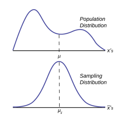
Notice that the horizontal axis in the top panel is labeled X. These are the individual observations of the population. This is the unknown distribution of the population values. The graph is purposefully drawn all squiggly to show that it does not matter just how odd ball it really is. Remember, we will never know what this distribution looks like, or its mean or standard deviation for that matter.
The horizontal axis in the bottom panel is labeled  . This is the theoretical distribution called the sampling distribution of the means. Each observation on this distribution is a sample mean. All these sample means were calculated from individual samples with the same sample size. The theoretical sampling distribution contains all of the sample mean values from all the possible samples that could have been taken from the population. Of course, no one would ever actually take all of these samples, but if they did this is how they would look. And the Central Limit Theorem says that they will be normally distributed.
The Central Limit Theorem goes even further and tells us the mean and standard deviation of this theoretical distribution.
| Parameter | Population distribution | Sample | Sampling distribution of  s s |
|---|---|---|---|
| Mean |  |
 |
 |
| Standard deviation |  |
s |  |
The practical significant of The Central Limit Theorem is that now we can compute probabilities for drawing a sample mean,  , in just the same way as we did for drawing specific observations,
  s, when we knew the population mean and standard deviation and that the population data were normally distributed. The standardizing formula has to be amended to recognize that the mean and standard deviation of the sampling distribution, sometimes, called the standard error of the mean, are different from those of the population distribution, but otherwise nothing has changed. The new standardizing formula is

Notice that in the first formula has been changed to simply in the second version. The reason is that mathematically it can be shown that the expected value of is equal to .
Sampling Distribution of the Sample Mean
Sampling Distribution of the Sample Mean (Part 2)
Sampling Distributions: Sampling Distribution of the Mean
Using the Central Limit Theorem
Law of Large Numbers
The law of large numbers says that if you take samples of larger and larger size from any population, then the mean of the sampling distribution, tends to get close and close to the true population mean, . From the Central Limit Theorem, we know that as n gets larger and larger, the sample means follow a normal distribution. The larger n gets, the smaller the standard deviation of the sampling distribution gets. (Remember that the standard deviation for sampling distribution of  . This means that the sample mean
  must be closer to the population mean as n increases. We can say that is the value that the sample means approach as n gets larger. The Central Limit Theorem illustrates the law of large numbers.
Indeed, there are two critical issues that flow from the Central Limit Theorem and the application of the Law of Large numbers to it. These are listed below.
-
- The probability density function of the sampling distribution of means is normally distributed regardless of the underlying distribution of the population observations and
- Standard deviation of the sampling distribution decreases as the size of the samples that were used to calculate the means for the sampling distribution increases.
Taking these in order. It would seem counterintuitive that the population may have any distribution and the distribution of means coming from it would be normally distributed. With the use of computers, experiments can be simulated that show the process by which the sampling distribution changes as the sample size is increased. These simulations show visually the results of the mathematical proof of the Central Limit Theorem.
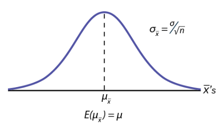
Figure 2 shows a sampling distribution. The mean has been marked on the horizontal axis of the  and the standard deviation has been written to the right above the distribution. Notice that the standard deviation of the sampling distribution is the original standard deviation of the population, divided by the sample size. We have already seen that as the sample size increases the sampling distribution becomes closer and closer to the normal distribution. As this happens, the standard deviation of the sampling distribution changes in another way; the standard deviation decreases as n increases. At very large n, the standard deviation of the sampling distribution becomes very small and at infinity it collapses on top of the population mean. This is what it means that the expected value of
  is the population mean, .
At non-extreme values of n, this relationship between the standard deviation of the sampling distribution and the sample size plays a very important part in our ability to estimate the parameters in which we are interested.
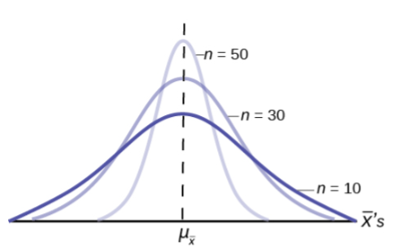
Figure 3 shows three sampling distributions. The only change that was made is the sample size that was used to get the sample means for each distribution. As the sample size increases, n goes from 10 to 30 to 50, the standard deviations of the respective sampling distributions decrease because the sample size is in the denominator of the standard deviations of the sampling distributions.
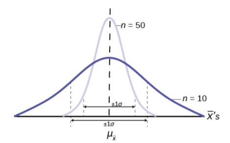
The implications for this are very important. Figure 4 shows the effect of the sample size on the confidence we will have in our estimates. These are two sampling distributions from the same population. One sampling distribution was created with samples of size 10 and the other with samples of size 50. All other things constant, the sampling distribution with sample size 50 has a smaller standard deviation that causes the graph to be higher and narrower. The important effect of this is that for the same probability of one standard deviation from the mean, this distribution covers much less of a range of possible values than the other distribution. One standard deviation is marked on the axis for each distribution. This is shown by the two arrows that are plus or minus one standard deviation for each distribution. If the probability that the true mean is one standard deviation away from the mean, then for the sampling distribution with the smaller sample size, the possible range of values is much greater. A simple question is, would you rather have a sample mean from the narrow, tight distribution, or the flat, wide distribution as the estimate of the population mean? Your answer tells us why people intuitively will always choose data from a large sample rather than a small sample. The sample mean they are getting is coming from a more compact distribution.
The Central Limit Theorem for Proportions
The Central Limit Theorem tells us that the point estimate for the sample mean, , comes from a normal distribution of . This theoretical distribution is called the sampling distribution of  . We now investigate the sampling distribution for another important parameter we wish to estimate, p from the binomial probability density function.
If the random variable is discrete, such as for categorical data, then the parameter we wish to estimate is the population proportion. This is, of course, the probability of drawing a success in any one random draw. Unlike the case just discussed for a continuous random variable where we did not know the population distribution of X’s, here we actually know the underlying probability density function for these data; it is the binomial. The random variable is X = the number of successes and the parameter we wish to know is p, the probability of drawing a success which is of course the proportion of successes in the population. The question at issue is: from what distribution was the sample proportion,  drawn? The sample size is n and X is the number of successes found in that sample. This is a parallel question that was just answered by the Central Limit Theorem: from what distribution was the sample mean, drawn? We saw that once we knew that the distribution was the Normal distribution then we were able to create confidence intervals for the population parameter, . We will also use this same information to test hypotheses about the population mean later. We wish now to be able to develop confidence intervals for the population parameter “p” from the binomial probability density function.
In order to find the distribution from which sample proportions come we need to develop the sampling distribution of sample proportions just as we did for sample means. So again, imagine that we randomly sample say 50 people and ask them if they support the new school bond issue. From this we find a sample proportion, p’, and graph it on the axis of p’s. We do this again and again etc., etc. until we have the theoretical distribution of p’s. Some sample proportions will show high favorability toward the bond issue and others will show low favorability because random sampling will reflect the variation of views within the population. What we have done can be seen in Figure 5. The top panel is the population distributions of probabilities for each possible value of the random variable X. While we do not know what the specific distribution looks like because we do not know p, the population parameter, we do know that it must look something like this. In reality, we do not know either the mean or the standard deviation of this population distribution, the same difficulty we faced when analyzing the X’s previously.
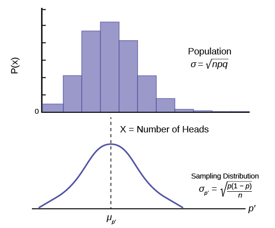
Figure 5 places the mean on the distribution of population probabilities as  but of course we do not actually know the population mean because we do not know the population probability of success, p. Below the distribution of the population values is the sampling distribution of p’s. Again, the Central Limit Theorem tells us that this distribution is normally distributed just like the case of the sampling distribution for . This sampling distribution also has a mean, the mean of the p’s, and a standard deviation,
  .
.
Importantly, in the case of the analysis of the distribution of sample means, the Central Limit Theorem told us the expected value of the mean of the sample means in the sampling distribution, and the standard deviation of the sampling distribution. Again, the Central Limit Theorem provides this information for the sampling distribution for proportions. The answers are:
-
- The expected value of the mean of sampling distribution of sample proportions,
 , is the population proportion, p.
 - The standard deviation of the sampling distribution of sample proportions, , is the population standard deviation divided by the square root of the sample size, n.
- The expected value of the mean of sampling distribution of sample proportions,
Both these conclusions are the same as we found for the sampling distribution for sample means. However, in this case, because mean and standard deviation of the binomial distribution both rely upon p, the formula for the standard deviation of the sampling distribution requires algebraic manipulation to be useful. The standard deviation of the sampling distribution for proportions is thus:

| Parameter | Population distribution | Sample | Sampling distribution of p‘s |
|---|---|---|---|
| Mean | |
|
 |
| Standard deviation |  |
 |
Table 2 summarizes these results and shows the relationship between the population, sample, and sampling distribution.
Reviewing the formula for the standard deviation of the sampling distribution for proportions we see that as n increases the standard deviation decreases. This is the same observation we made for the standard deviation for the sampling distribution for means. Again, as the sample size increases, the point estimate for either  is found to come from a distribution with a narrower and narrower distribution. We concluded that with a given level of probability, the range from which the point estimate comes is smaller as the sample size, n, increases.
Find Confidence Intervals for Parameter Estimates
In this section, you will learn how to find and estimate confidence intervals by reading each description along with watching the videos included. Also, short problems to check your understanding are included.
Confidence Intervals & Estimation: Point Estimates Explained
Introduction to Confidence Intervals
Suppose you were trying to determine the mean rent of a two-bedroom apartment in your town. You might look in the classified section of the newspaper, write down several rents listed, and average them together. You would have obtained a point estimate of the true mean. If you are trying to determine the percentage of times you make a basket when shooting a basketball, you might count the number of shots you make and divide that by the number of shots you attempted. In this case, you would have obtained a point estimate for the true proportion the parameter p in the binomial probability density function.
We use sample data to make generalizations about an unknown population. This part of statistics is called inferential statistics. The sample data help us to make an estimate of a population parameter. We realize that the point estimate is most likely not the exact value of the population parameter, but close to it. After calculating point estimates, we construct interval estimates, called confidence intervals. What statistics provides us beyond a simple average, or point estimate, is an estimate to which we can attach a probability of accuracy, what we will call a confidence level. We make inferences with a known level of probability.
If you worked in the marketing department of an entertainment company, you might be interested in the mean number of songs a consumer downloads a month from iTunes. If so, you could conduct a survey and calculate the sample mean, , and the sample standard deviation, s. You would use to estimate the population mean and s to estimate the population standard deviation. The same mean, , is the point estimate for the population mean, . The sample standard deviation, s, is the point estimate for the population standard deviation, .
and s are each called a statistic.
A confidence interval is another type of estimate but, instead of being just one number, it is an interval of numbers. The interval of numbers is a range of values calculated from a given set of sample data. The confidence interval is likely to include the unknown population parameter.
Suppose for the iTunes examples, we do not know the population mean , but we do know that the population standard deviation is  and our sample size is 100. Then, by the Central Limit Theorem, the standard deviation of the sampling distribution of the sample means is
  .
.
The Empirical Rule, which applies to the normal distribution, says that in approximately 95% of the samples, the same mean, , will be within two standard deviations of the population mean  . For our iTunes example, two standard deviations is
  . The sample mean is likely to be within 0.2 units of .
Because is within 0.2 units of  which is unknown, then is likely to be within 0.2 units of with 95% probability. The population mean is contained in an interval whose lower number is calculated by taking the sample mean and subtracting two standard deviations
  and whose upper number is calculated by taking the sample mean and adding two standard deviations. In other words, is between
  in 955 of all the samples.
For the iTunes example, suppose that a sample produced a sample mean  . Then with 95% probability the unknown population mean is between

We say that we are 95% confident that the unknown population mean number of songs downloaded from iTunes per month is between 1.8 and 2.2. The 95% confidence interval is (1.8, 2.2). Please note that we talked in terms of 95% confidence using the empirical rule. The empirical rule for two standard deviations is only approximately 95% of the probability under the normal distribution. To be precise, two standard deviations under a normal distribution is actually 95.44% of the probability. To calculate the exact 95% confidence level, we would use 1.96 standard deviations.
The 95% confidence interval implies two possibilities. Either the interval (1.8, 2.2) contains the true mean 𝜇, or our sample produce an that is not within 0.2 units of the true mean 𝜇. The first possibility happens for 95% of well-chosen samples. It is important to remember that the second possibility happens for 5% of samples, even though correct procedures are followed.
Remember that a confidence interval is created for an unknown population parameter like the population mean, 𝜇.
For the confidence interval for a mean the formula would be:

Or written another way as:

Where s is the sample mean.  a is determined by the level of confidence desired by the analyst, and
  is the standard deviation of the sampling distribution for means given to us by the Central Limit Theorem.
A Confidence Interval for a Population Standard Deviation, Known or Large Sample Size
A confidence interval for a population mean, when the population standard deviation is known based on the conclusion of the Central Limit Theorem that the sampling distribution of the sample means follow an approximately normal distribution.
Calculating the Confidence Interval
Consider the standardizing formula for the sampling distribution developed in the discussion of the Central Limit Theorem:

Notice that is substituted for  – because we know that the expected value of – is from the Central Limit Theorem and
  – is replaced with , also from the Central Limit Theorem.
In this formula we know  and n, the sample size. (In actuality we do not know the population standard deviation, but we do have a point estimate for it, s, from the sample we took. More on this later.) What we do not know is
  We can solve for either one of these in terms of the other. Solving for 𝜇 in terms of
  gives:

Remembering that the Central Limit Theorem tells us that the distribution of the  , the sampling distribution for means, is normal, and that the normal distribution is symmetrical, we can rearrange terms thus:

This is the formula for a confidence interval for the mean of a population.
Notice that  has been substituted for
  in this equation. This is where the statistician must make a choice. The analyst must decide the level of confidence they wish to impose on the confidence interval.
  is the probability that the interval will not contain the true population mean. The confidence level is defined as
  is the number of standard deviations lies from the mean with a certain probability. If we chose,
  we are asking for the 95% confidence interval because we are setting the probability that the true mean lies within the range at 0.95. If we set at 1.64 we are asking for the 90% confidence interval because we have set the probability at 0.90. These numbers can be verified by consulting the Standard Normal table. Divide either 0.95 or 0.90 in half and find that probability inside the body of the table. Then read on the top and left margins the number of standard deviations it takes to get this level of probability.
| Confidence Level | blank cell |
|---|---|
| 0.80 | 1.28 |
| 0.90 | 1.645 |
| 0.95 | 1.96 |
| 0.99 | 2.58 |
In reality, we can set whatever level of confidence we desire simply by changing the value in the formula. It is the analyst’s choice. Common convention in Economics and most social sciences sets confidence intervals at either 90, 95, or 99 percent levels. Levels less than 90% are considered of little value. The level of confidence of a particular interval estimate is called  .
.
Let us say we know that the actual population mean number of iTunes downloads is 2.1. The true population mean falls within the range of the 95% confidence interval. There is absolutely nothing to guarantee that this will happen. Further, if the true mean falls outside of the interval, we will never know it. We must always remember that we will never ever know the true mean. Statistics simply allows us, with a given level of probability (confidence), to say that the true mean is within the range calculated.
Changing the Confidence Level or Sample Size
Here again is the formula for a confidence interval for an unknown population mean assuming we know the population standard deviation:

It is clear that the confidence interval is driven by two things, the chosen level of confidence, , and the standard deviation of the sampling distribution. The standard deviation of the sampling distribution is further affected by two things, the standard deviation of the population and sample size we chose for our data. Here we wish to examine the effects of each of the choices we have made on the calculated confidence interval, the confidence level, and the sample size.
For a moment we should ask just what we desire in a confidence interval. Our goal was to estimate the population mean from a sample. We have forsaken the hope that we will ever find the true population mean, and population standard deviation for that matter, for any case except where we have an extremely small population and the cost of gathering the data of interest is very small. In all other cases we must rely on samples. With the Central Limit Theorem, we have the tools to provide a meaningful confidence interval with a given level of confidence, meaning a known probability of being wrong. By meaningful confidence interval we mean one that is useful. Imagine that you are asked for a confidence interval for the ages of your classmates. You have taken a sample and find a mean of 19.8 years. You wish to be very confident, so you report an interval between 9.8 years and 29.8 years. This interval would certainly contain the true population mean and have a very high confidence level. However, it hardly qualifies as meaningful. The very best confidence interval is narrow while having high confidence. There is a natural tension between these two goals. The higher the level of confidence the wider the confidence interval as the case of the students’ ages above. We can see this tension in the equation for the confidence interval.

The confidence interval will increase in width as increases, increases as the level of confidence increases. There is a tradeoff between the level of confidence and the width of the interval. Now let us look at the formula again and we see that the sample size also plays an important role in the width of the confidence interval. The sample size, n, shows up in the denominator of the standard deviation of the sampling distribution. As the sample size increases, the standard deviation of the sampling distribution decreases and thus the width of the confidence interval, while holding constant the level of confidence. Again, we see the importance of having large samples for our analysis although we then face a second constraint, the cost of gathering data.
Calculating the Confidence Interval: An Alternative Approach
Another way to approach confidence intervals is through the use of something called the Error Bound (margin of error). The Error Bound gets its name from the recognition that it provides the boundary of the interval derived from the standard error of the sampling distribution. In the equations above it is seen that the interval is simply the estimated mean, sample mean, plus or minus something. That something is the Error Bound and is driven by the probability we desire to maintain in our estimate, , times the standard deviation of the sampling distribution. The Error Bound for a mean is given the name, Error Bound Mean, or EBM (or margin of error, M.O.E.).
To construct a confidence interval for a single unknown population, mean 𝜇, where the population standard deviation is known, we need as an estimate for 𝜇 and we need the margin of error. Here, the margin of error (EBM) is called the error bound for a population mean. The sample mean is the point estimate of the unknown population mean 𝜇.
The confidence interval estimate will have the form:
(Point estimate – error bound, point estimate + error bound) or, in symbols,

The mathematical formula for this confidence interval is:
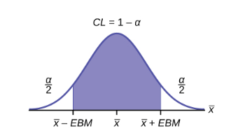
The margin of error (EBM) depends on the confidence level (abbreviated CL). The confidence level is often considered the probability that the calculated confidence interval estimate will contain the true population parameter. However, it is more accurate to state that the confidence level is the percent of confidence intervals that contain the true population parameter when repeated samples are taken. Most often, it is the choice of the person constructing the confidence interval to choose a confidence level of 90% or higher because that person wants to be reasonably certain of his or her conclusions.
There is another probability called alpha  is related to the confidence level, CL. is the probability that the interval does not contain the unknown population parameter. Mathematically,
  .
.
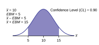
A confidence interval for a population mean with a known standard deviation is based on the fact that the sampling distribution of the sample means follow an approximately normal distribution. Suppose that our sample has a mean of  and we have constructed the 90% confidence interval (5, 15) where EMB = 5.
To get a 90% confidence interval, we must include the central 90% of the probability of the normal distribution. If we include the central 90%, we leave out a total of  in both tails, or 5% in each tail, of the normal distribution.
To capture the central 90%, we must go out 1.645 standard deviations on either side of the calculated sample mean. The value 1.645 is the z-score from a standard normal probability distribution that puts an area of 0.90 in the center, an area of 0.05 in the far-left tail, and an area of 0.05 in the far-right tail.
It is important that the standard deviation used must be appropriate for the parameter we are estimating, so in this section we need to use the standard deviation that applies to the sampling distribution for mean which we studied with the Central Limit Theorem and is,  .
.
Calculating the Confidence Interval Using EBM
To construct a confidence interval, estimate for an unknown population mean, we need data from a random sample. The steps to construct and interpret the confidence interval are listed below.
- Calculate the sample mean from the sample data. Remember, in this section we know the population standard deviation .
- Find the z-score from the standard normal table that corresponds to the confidence level desired.
- Calculate the error bound EBM.
- Construct the confidence interval.
- Write a sentence that interprets the estimate in the context of the situation in the problem.
Finding the z-score for the Stated Confidence Level
When we know the population standard deviation , we use a standard normal distribution to calculate the error bound EBM and construct the confidence interval. We need to find the value of z that puts an area equal to the confidence level (in decimal form) in the middle of the standard normal distribution  .
.
The confidence level, CL, is the area in the middle of the standard normal distribution.  is the area that is split equally between the two tails. Each of the tails contains an area equal to
  .
.
The z-score that has an area to the right of is denoted by 
For example, when 
The area to the right of  is
is  .
.
 , using a standard normal probability table. We will see later that we can use a different probability table, the Student's t-distribution, for finding the number of standard deviations of commonly used levels of confidence.
Calculating the Error Bound (EBM)
The error bound formula for an unknown population mean when the population standard deviation is known as

Constructing the Confidence Interval
The confidence interval estimate has the format  or the formula:

The graph gives a picture of the entire situation.

Confidence Interval for Mean: 1 Sample Z Test (Using Formula)
Check Your Understanding: Confidence Interval for Mean
A Confidence Interval for a Population Standard Deviation Unknown, Small Sample Case
In practice, we rarely known the population standard deviation. In the past, when the sample size was large, this did not present a problem to statisticians. They used the sample standard deviation s as an estimate for and proceeded as before to calculate a confidence interval with close enough results. Statisticians ran into problems when the sample size was small. A small sample size caused inaccuracies in the confidence interval.
William S. Goset (1876-1937) of the Guinness brewery in Dublin, Ireland ran into this problem. His experiments with hops and barely produced very few samples. Just replacing with s did not produce accurate results when he tried to calculate a confidence interval. He realized that he could not use a normal distribution for the calculation; he found that the actual distribution depends on the sample size. This problem led him to “discover” what is called the Student’s t-distribution. The name comes from the fact that Gosset wrote under the pen name “A Student.”
Up until the mid-1970s, some statisticians used the normal distribution approximation for large sample sizes and used the Student’s t-distribution only for sample sizes of at most 30 observations.
If you draw a simple random sample of size n from a population with mean 𝜇 and unknown population standard deviation and calculate the t-score  , then the t-scores follow a Student’s t-distribution with n – 1 degrees of freedom. The t-score has the same interpretation as the z-score. It measures how far in standard deviation units is from its mean . For each sample size n, there is a different Student’s t-distribution.
The degrees of freedom, n – 1, come from the calculation of the sample standard deviation s. Remember when we first calculated a sample standard deviation, we divided the sum of the squared deviations by  , but we used n deviations
  to calculate s. Because the sum of the deviations is zero, we can find the last deviation once we know the other deviations. The other deviations can change or vary freely. We call the number the degrees of freedom (df) in recognition that one is lost in the calculations. The effect of losing a degree of freedom is that the t-value increases, and the confidence interval increases in width.
Properties of the Student’s t-distribution
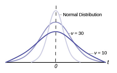
- The graph for the Student’s t-distribution is similar to the standard normal curve and at infinite degrees of freedom it is the normal distribution. You can confirm this by reading the bottom line at infinite degrees of freedom for a familiar level of confidence, e.g., at column 0.05, 95% level of confidence, we find the t-value of 1.96 at infinite degrees of freedom.
- The mean for the Student’s t-distribution is zero and the distribution is symmetric about zero, again like the standard normal distribution.
- The Student’s t-distribution has more probability in its tails than the standard normal distribution because the spread of the t-distribution is greater than the spread of the standard normal. So, the graph of the Student’s t-distribution will be thicker in the tails and shorter in the center than the graph of the standard normal distribution.
- The exact shape of the Student’s t-distribution depends on the degrees of freedom. As the degrees of freedom increases, the graph of Student’s t-distribution becomes more like the graph of the standard normal distribution.
- The underlying population of individual observations is assumed to be normally distributed with unknown population mean and unknown population standard deviation 𝜎. This assumption comes from the Central Limit Theorem because the individual observations in this case are the of the sample distribution. The size of the underlying population is generally not relevant unless it is very small. If it is normal, then the assumption is met and does not need discussion.
A probability table for the Student’s t-distribution is used to calculate t-values at various commonly used levels of confidence. The table gives t-scores that correspond to the confidence level (column) and degrees of freedom (row). When using a t-table, note that some tables are formatted to show the confidence level in the column headings, while the column headings in some tables may show only corresponding area in one or both tails. Notice that at the bottom the table will show the t-value for infinite degrees of freedom. Mathematically, as the degrees of freedom increase, the t-distribution approaches the standard normal distribution. You can find familiar Z-values by looking in the relevant alpha column and reading value in the last row.
A Student’s t-table gives t-scores given the degrees of freedom and the right-tailed probability.
The Student’s t-distribution has one of the most desirable properties of the normal: it is symmetrical. What the Student’s t-distribution does is spread out the horizontal axis, so it takes a larger number of standard deviations to capture the same amount of probability. In reality there are an infinite number of Student’s t-distributions, one for each adjustment to the sample size. As the sample size increases, the Student’s t-distribution become more and more like the normal distribution. When the sample size reaches 30 the normal distribution is usually substituted for the Student’s t because they are so much alike. This relationship between the Student’s t-distribution and the normal distribution is shown in Figure 8.
Here is the confidence interval for the mean for cases when the sample size is smaller than 30 and we do not know the population standard deviation, :

Here the point estimate of the population standard deviation, s has been substituted for the population standard deviation, , and  has been substituted for
  . The Greek letter
  (pronounced nu) is places in the general formula in recognition that there are many Student
  distributions, one for each sample size.
  is the symbol for the degrees of freedom of the distribution and depends on the size of the sample. Often df is used to abbreviate degrees of freedom. For this type of problem, the degrees of freedom is
  , where n is the sample size. To look up a probability in the Student’s t table we have to know the degrees of freedom in the problem.
Confidence Intervals: Using the t Distribution
Check Your Understanding: Confidence Intervals
A Confidence Interval for a Population Proportion
During an election year, we see articles in the newspaper that state confidence intervals in terms of proportions or percentages. For example, a poll for a particular candidate running for president might show that the candidate has 40% of the vote within three percentage points (if the sample is large enough). Often, election polls are calculated with 95% confidence, so, the pollsters would be 95% confident that the true proportion of voters who favored the candidate would be between 0.37 and 0.43.
The procedure to find the confidence interval for a population proportion is similar to that for the population mean, but the formulas are a bit different although conceptually identical. While the formulas are different, they are based upon the same mathematical foundation given to us by the Central Limit Theorem. Because of this we will see the same basic format using the same three pieces of information: the sample value of the parameter in question, the standard deviation of the relevant sampling distribution, and the number of standard deviations we need to have the confidence in our estimate that we desire.
How do you know you are dealing with a proportion problem? First, the underlying distribution has a binary random variable and therefore is a binomial distribution. (There is no mention of a mean or average). If X is a binomial random variable, then  where n is the number of trials and p is the probability of a success. To form a sample proportion, take X, the random variable for the number of successes and divide it by n, the number of trials (or the sample size). The random variable
  (read “P Prime”) is the sample proportion,

(Sometimes the random variable is denoted as  , read “P hat.”)
 = the estimated proportion of successes or sample proportion of successes (p’ is a point estimate for p, the true population proportion, and thus q is the probability of a failure in any one trial.)
x = the number of successes in the sample
n = the size of the sample
The formula for the confidence interval for a population proportion follows the same format as that for an estimate of a population mean. Remembering the sampling distribution for the proportion, the standard deviation was found to be:

The confidence interval for a population proportion, therefore, becomes:
![p=p^{\prime} \pm\left[Z_{\left(\frac{\alpha}{2}\right)} \sqrt{\frac{p^{\prime}\left(1-p^{\prime}\right)}{n}}\right]](https://uta.pressbooks.pub/app/uploads/quicklatex/quicklatex.com-15669649a79636d094614c8b9359348a_l3.png "Rendered by QuickLaTeX.com")
 is set according to our desired degree of confidence and
  is the standard deviation of the sampling distribution.
The sample proportions p’ and q’ are estimates of the unknown population proportions p and q. The estimated proportions p’ and q’ are used because p and q are not known.
Remember that as p moves further from 0.5 the binomial distribution becomes less symmetrical. Because we are estimating the binomial with the symmetrical normal distribution the further away from symmetrical the binomial becomes the less confidence we have in the estimate.
This conclusion can be demonstrated through the following analysis. Proportions are based upon the binomial probability distribution. The possible outcomes are binary, either “success” or “failure.” This gives rise to a proportion, meaning the percentage of the outcomes that are “successes.” It was shown that the binomial distribution could be fully understood if we knew only the probability of a success in any one trial, called p. The mean and the standard deviation of the binomial were found to be:
It was also shown that the binomial could be estimated by the normal distribution if BOTH np AND nq were greater than 5. From the discussion above, it was found that the standardizing formula for the binomial distribution is:

Which is nothing more than a restatement of the general standardizing formula with appropriate substitutions for and from the binomial. We can use the standard normal distribution, the reason Z is in the equation, because the normal distribution is the limiting distribution of the binomial. This is another example of the Central Limit Theorem.
We can now manipulate this formula in just the same way we did for finding the confidence intervals for a mean, but to find the confidence interval for the binomial population parameter, p.

Where  , the point estimate of p taken from the sample. Notice that p’ has replaced p in the formula. This is because we do not know p, indeed, this is just what we are trying to estimate.
x = number of successes.
n = the number in the sample.
 , the failure in any trial
Unfortunately, there is no correction factor for cases where the sample size is small so np’ and nq’ must always be greater than 5 to develop an interval estimate for p.
Also written as:

How to Construct a Confidence Interval for Population Proportion
Check Your Understanding: How to Construct a Confidence Interval for Population Proportion
Estimate the Required Sample Size for Testing
In this section, you will learn how to calculate sample size with continuous and binary random samples. by reading each description along with watching the videos included. Also, short problems to check your understanding are included.
Calculating the Sample Size n: Continuous and Binary Random Variables
Continuous Random Variables
Usually, we have no control over the sample size of a data set. However, if we are able to set the sample size, as in cases where we are taking a survey, it is very helpful to know just how large it should be to provide the most information. Sampling can be very costly in both time and product. Simple telephone surveys will cost approximately $30.00 each, for example, and some sampling requires the destruction of the product.
If we go back to our standardizing formula for the sampling distribution for means, we can see that it is possible to solve it for n. If we do this, we have  in the denominator.

Because we have not taken a sample, yet we do not know any of the variables in the formula except that we can set to the level of confidence we desire just as we did when determining confidence intervals. If we set a predetermined acceptable error, or tolerance, for the difference between  in the formula, we are much further in solving for the sample size n. We still do not know the population standard deviation, . In practice, a pre-survey is usually done which allows for fine tuning the questionnaire and will give a sample standard deviation that can be used. In other cases, previous information from other surveys may be used for in the formula. While crude, this method of determining the sample size may help in reducing cost significantly. If will be the actual data gathered that determines the inferences about the population, so caution in the sample size is appropriate calling for high levels of confidence and small sampling errors.
Binary Random Variables
What was done in cases when looking for the mean of a distribution can also be done when sampling to determine the population parameter p for proportions. Manipulation of the standardizing formula for proportions gives:

Where  , and is the acceptable sampling error, or tolerance, for this application. This will be measured in percentage points.
In this case the very object of our search is in the formula, p, and of course q because  . This result occurs because the binomial distribution is a one parameter distribution. If we know p then we know the mean and the standard deviation. Therefore, p shows up in the standard deviation of the sampling distribution which is where we got this formula. If, in an abundance of caution, we substitute 0.5 for p we will draw the largest required sample size that will provided the level of confidence specified by and the tolerance we have selected. This is true because of all combinations of two fractions that add to one, the largest multiple is when each is 0.5. Without any other information concerning the population parameter p, this is the common practice. This may result in oversampling, but certainly not under sampling, thus, this is a cautious approach.
There is an interesting trade-off between the level of confidence and the sample size that shows up here when considering the cost of sampling. Table 4 shows the appropriate sample size at different levels of confidence and different level of the acceptable error, or tolerance.
| Required sample size (90%) | Required sample size (95%) | Tolerance level |
|---|---|---|
| 1691 | 2401 | 2% |
| 752 | 1067 | 3% |
| 271 | 384 | 5% |
| 68 | 96 | 10% |
Table 4 is designed to show the maximum sample size required at different levels of confidence given an assumed  as discussed above.
The acceptable error, called tolerance in the table, is measured in plus or minus values from the actual proportion. For example, an acceptable error of 5% means that if the sample proportion was found to be 26 percent, the conclusion would be that the actual population proportion is between 21 and 31 percent with a 90 percent level of confidence if a sample of 271 had been taken. Likewise, if the acceptable error was set at 2%, then the population proportion would be between 24 and 28 percent with a 90 percent level of confidence but would require that the sample size be increased from 271 to 1,691. If we wished a higher level of confidence, we would require a larger sample size. Moving from a 90 percent level of confidence to a 95 percent level at a plus or minus 5% tolerance requires changing the sample size from 271 to 384. A very common sample size often seen reported in political surveys is 384. With the survey results it is frequently stated that the results are good to a plus or minus 5% level of “accuracy”.
Example: Suppose a mobile phone company wants to determine the current percentage of customers aged 50+ who use text messaging on their cell phones. How many customers aged 50+ should the company survey in order to be 90% confident that the estimated (sample) proportion is within three percentage points of the true population proportion of customers aged 50+ who use text messaging on their cell phones.
Solution: From the problem, we know that the acceptable error, e, is 0.03 (3% = 0.03) and  , because the confidence level is 90%. The acceptable error, e, is the difference between the actual population proportion p, and the sample proportion we expect to get from the sample.
However, in order to find n, we need to know the estimated (sample) proportion p’. Remember that  . But we do not know p’ yet. Since we multiply p’ and q’ together, we make them both equal to 0.5 because
  results in the largest possible product. (Try other products:
  and so on). The largest possible product gives us the largest n. This gives us a large enough sample so that we can be 90% confident that we are within three percentage points of the true population proportion. To calculate the sample size n, use the formula and make the substitutions.

Round the answer to the next higher value. The sample size should be 752 cell phone customers aged 50+ in order to be 90% confident that the estimated (sample) proportion is within three percentage points of the true population proportion of all customers aged 50+ who use text messaging on their cell phones.
Estimation and Confidence Intervals: Calculate Sample Size
Calculating Sample size to Predict a Population Proportion
Use Specific Significance Tests Including, Z-Test, T-Test (one and two samples), Chi-Squared Test
In this section, you will learn the fundamentals of hypothesis testing along with hypothesis testing with errors by reading each description along with watching the videos. Also, short problems to check your understanding are included.
Hypothesis Testing with One Sample
Statistical testing is part of a much larger process known as the scientific method. The scientific method, briefly, states that only by following a careful and specific process can some assertion be included in the accepted body of knowledge. This process begins with a set of assumptions upon which a theory, sometimes called a model, is built. This theory, if it has any validity, will lead to predictions; what we call hypotheses.
Statistics and statisticians are not necessarily in the business of developing theories, but in the business of testing others’ theories. Hypotheses come from these theories based upon an explicit set of assumptions and sound logic. The hypothesis comes first, before any data are gathered. Data do not create hypotheses; they are used to test them. If we bear this in mind as we study this section, the process of forming and testing hypotheses will make more sense.
One job of a statistician is to make statistical inferences about populations based on samples taken from the population. Confidence intervals are one way to estimate a population parameter. Another way to make a statistical inference is to make a decision about the value of a specific parameter. For instance, a car dealer advertises that its new small truck gets 35 miles per gallon, on average. A tutoring service claims that its method of tutoring helps 90% of its students get an A or a B. A company says that women managers in their company earn an average of $60,000 per year.
A statistician will make a decision about these claims. This process is called "hypothesis testing." A hypothesis test involves collecting data from a sample and evaluating the data. Then, the statistician makes a decision as to whether or not there is sufficient evidence, based upon analyses of the data, to reject the null hypothesis.
Hypothesis Testing: The Fundamentals
Null and Alternative Hypotheses
The actual test begins by considering two hypotheses. They are called the null hypothesis and the alternative hypothesis. These hypotheses contain opposing viewpoints.
 The null hypothesis: It is a statement of no difference between the variables–they are not related. This can often be considered the status quo and as a result if you cannot accept the null, it requires some action.
 The alternative hypothesis: It is a claim about the population that is contradictory to
  and what we conclude when we cannot accept . This is usually what the researcher is trying to prove. The alternative hypothesis is the contender and must win with significant evidence to overthrow the status quo. This concept is sometimes referred to the tyranny of the status quo because as we will see later, to overthrow the null hypothesis takes usually 90 or greater confidence that this is the proper decision.
Since the null and alternative hypotheses are contradictory, you must examine evidence to decide if you have enough evidence to reject the null hypothesis or not. The evidence is in the form of sample data.
After you have determined which hypothesis the sample supports, you make a decision. There are two options for a decision. They are “cannot accept ” if the sample information favors the alternative hypothesis or “do not reject ” or “decline to reject ” if the sample information is insufficient to reject the null hypothesis. These conclusions are all based upon a level of probability, a significance level, that is set by the analyst.
Table 5 presents the various hypotheses in the relevant pairs. For example, if the null hypothesis is equal to some value, the alternative has to be not equal to that value.
|
 |
|---|---|
| Equal (=) | Not equal  |
Greater than or equal to  |
Less than (<) |
Less than or equal to  |
More than (>) |
Note: As a mathematical convention  always has a symbol with an equal in it. never has a symbol with an equal in it. The choice of symbol depends on the wording of the hypothesis test.
Example 1:
: No more than 30% of the registered voters in Santa Clara County voted in the primary election. 
: More than 30% of the registered voters in Santa Clara County voted in the primary election. 
Example 2: We wants to test whether the mean GPA of students in American colleges is different from 2.0 (out of 4.0). The null and alternative hypotheses are:


Example 3: We want to test if college students take less than five years to graduate from college, on the average. The null and alternative hypotheses are:


Hypothesis Testing: Setting up the Null and Alternative Hypothesis Statements
Outcomes and the Type I and Type II Errors
When you perform a hypothesis test, there are four possible outcomes depending on the actual truth (or falseness) of the null hypothesis  and the decision to reject or not. The outcomes are summarized in Table 6:
| Statistical Decision | is actually… |
blank cell |
|---|---|---|
| True | False | |
| Cannot reject |
Correct outcome | Type II error |
| Cannot accept |
Type I error | Correct outcome |
The four possible outcomes in the table are:
-
-
-
- The decision is cannot reject when is true (correct decision).
- The decision is cannot accept when is true (incorrect decision known as a Type I error). This case is described as “rejecting a good null”. As we will see later, it is this type of error that we will guard against by setting the probability of making such an error. The goal is to NOT take an action that is an error.
- The decision is cannot reject when, in fact, is false (incorrect decision known as a Type II error). This is called “accepting a false null”. In this situation you have allowed the status quo to remain in force when it should be overturned. As we will see, the null hypothesis has the advantage in competition with the alternative.
- The decision is cannot accept when is false (correct decision).
- The decision is cannot reject
-
-
Each of the errors occurs with a particular probability. The Greek letters and  represent the probabilities.
 probability of a Type I error = P(Type I error) = probability of rejecting the null hypothesis when the null hypothesis is true: rejecting a good null.
 probability of a Type II error = P(Type II error) = probability of not rejecting the null hypothesis when the null hypothesis is false.
  is called the Power of the Test.
 should be as small as possible because they are probabilities of errors.
Statistics allows us to set the probability that we are making a Type I error. The probability of making a Type I error is . Recall that the confidence intervals in the last section were set by choosing a value called  and the alpha value determined the confidence level of the estimate because it was the probability of the interval failing to capture the true mean (or proportion parameter p). This alpha and that one are the same.
The easiest way to see the relationship between the alpha error and the level of confidence is in Figure 9.
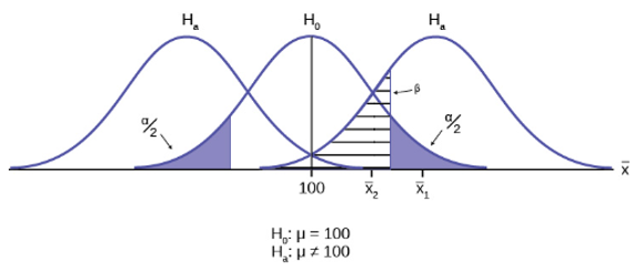
In the center of Figure 9 is a normally distributed sampling distribution marked . This is a sampling distribution of and by the Central Limit Theorem it is normally distributed. The distribution in the center is marked and represents the distribution for the null hypotheses  . This is the value that is being tested. The formal statements of the null and alternative hypotheses are listed below the figure.
The distributions on either side of the distribution represent distributions that would be true if is false, under the alternative hypothesis listed as . We do not know which is true, and will never know. There are, in fact, an infinite number of distributions from which the data could have been drawn if is true, but only two of them are on Figure 9 representing all of the others.
To test a hypothesis, we take a sample from the population and determine if it could have come from the hypothesized distribution with an acceptable level of significance. This level of significance is the alpha error and is marked on Figure 9 as the shaded areas in each tail of the distribution. (Each are actually  because the distribution is symmetrical, and the alternative hypothesis allows for the possibility for the value to be either greater than or less than the hypothesized value–called a two-tailed test).
If the sample mean marked as  is in the tail of the distribution of , we conclude that the probability that it could have come from the distribution is less than alpha. We consequently state, “the null hypothesis cannot be accepted with
  level of significance.” The truth may be that this did come from the distribution, but from out in the tail. If this is so, then we have falsely rejected a true null hypothesis and have made a Type I error. What statistics has done is provide an estimate about what we know, and what we control, and that is the probability of us being wrong, .
We can also see in Figure 9 that the sample mean could be really from an  distribution, but within the boundary set by the alpha level. Such a case is marked as
  . There is a probability that actually came from but shows up in the range of between the two tails. This probability is the beta error, the probability of accepting a false null.
Our problem is that we can only set the alpha error because there are an infinite number of alternative distributions from which the mean could have come that are not equal to . As a result, the statistician places the burden of proof on the alternative hypothesis. That is, we will not reject a null hypothesis unless there is a greater than 90, or 95, or even 99 percent probability that the null is false: the burden of proof lies with the alternative hypothesis. This is why we called this the tyranny of the status quo earlier.
By way of example, the American judicial system begins with the concept that a defendant is “presumed innocent”. This is the status quo and is the null hypothesis. The judge will tell the jury that they cannot find the defendant guilty unless the evidence indicates guilt beyond a “reasonable doubt” which is usually defined in criminal cases as 95% certainty of guilt. If the jury cannot accept the null, innocent, then action will be taken, jail time. The burden of proof always lies with the alternative hypothesis. (In civil cases, the jury needs only to be more than 50% certain of wrongdoing to find culpability, called “a preponderance of the evidence”).
The example above was for a test of a mean, but the same logic applies to tests of hypotheses for all statistical parameters one may wish to test.
Example: Suppose the null hypothesis, , is Frank’s rock climbing is safe.
Type I error: Frank thinks that his rock-climbing equipment may not be safe when, in fact, it really is safe.
Type II error: Frank thinks that his rock-climbing equipment may be safe when, in fact, it is not safe.
probability that Frank thinks his rock-climbing equipment may not be safe when, in fact, it really is safe.  probability that Frank thinks his rock-climbing equipment may be safe when, in fact, it is not safe.
Notice that, in this case, the error with the greater consequence is the Type II error. (If Frank thinks his rock-climbing equipment is safe, he will go ahead and use it.)
This is a situation described as “accepting a false null”.
Hypothesis Testing: Type I and Type II Errors
Check Your Understanding: Hypothesis Testing: Type I and Type II Errors
Distribution Needed for Hypothesis Testing
Earlier, we discussed sampling distributions. Particular distributions are associated with hypothesis testing. We will perform hypotheses tests of a population mean using a normal distribution or a Student’s t-distribution. (Remember, use a Student’s t-distribution when the population standard deviation is unknown and the sample size is small, where small is considered to be less than 30 observations.) We perform tests of a population proportion using a normal distribution when we can assume that the distribution is normally distributed. We consider this to be true if the sample proportion, p’, times the sample size is greater than 5 and  times the sample size is also greater than 5. This is the same rule of thumb we used when developing the formula for the confidence interval for a population proportion.
Hypothesis Test for the Mean
Going back to the standardizing formula we can derive the test statistic for testing hypotheses concerning means.

The standardizing formula cannot be solved as it is because we do not have , the population mean. However, if we substituted in the hypothesized value of the mean,  in the formula as above, we can compute a Z value. This is the test statistic for a test of hypothesis for a mean and is presented in Figure 10. We interpret this Z value as the associated probability that a sample with a sample mean of could have come from a distribution with a population mean of and we call this Z value
  for “calculated.” Figure 10 shows this process.
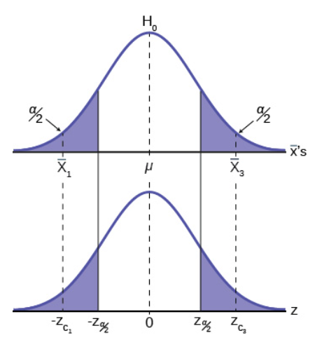
In Figure 10, two of the three possible outcomes are presented. and  are in the tails of the hypothesized distribution of . Notice that the horizontal axis in the top panel is labeled
  s. This is the same theoretical distribution of
  , the sampling distribution, that the Central Limit Theorem tells us is normally distributed. This is why we can draw it with this shape. The horizontal axis of the bottom panel is labeled Z and is the standard normal distribution.
  , called the critical values, are marked on the bottom panel as the Z values associated with the probability the analyst has set as the level of significance in test, . The probabilities in the tails of both panels are, therefore, the same.
Notice that for each there is an associated , called the calculated Z, that comes from solving the equation above. This calculated Z is nothing more than the number of standard deviations that the hypothesized mean is from the sample mean. If the sample mean falls “too many” standard deviations from the hypothesized mean we conclude that the sample mean could not have come from the distribution with the hypothesized mean, given our pre-set required level of significance. It could have come from , but it is deemed just too unlikely. In Figure 10, both  are in the tails of the distribution. They are deemed “too far” from the hypothesized value of the mean given the chosen level of alpha. If in fact this sample mean it did come from , but from in the tail, we have made a Type I error: we have rejected a good null. Our only real comfort is that we know the probability of making such an error, , and we can control the size of .
Figure 11 shows the third possibility for the location of the sample mean, . Here the sample mean is within the two critical values. That is, within the probability of  and we cannot reject the null hypothesis.
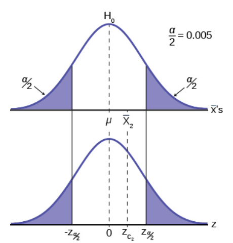
This gives us the decision rule for testing a hypothesis for a two-tailed test:
| Decision rule: two-tail test |
|---|
If  : then DO NOT REJECT : then DO NOT REJECT |
If  : then REJECT : then REJECT |
This rule will always be the same no matter what hypothesis we are testing or what formulas we are using to make the test. The only change will be change the to the appropriate symbol for the test statistic for the parameter being tested. Stating the decision rule another way: if the sample mean is unlikely to have come from the distribution with the hypothesized mean we cannot accept the null hypothesis. Here we define “unlikely” as having a probability less than alpha of occurring.
Hypothesis testing: Finding Critical Values
Normal Distribution: Finding Critical Values of Z
P-Value Approach
An alternative decision rule can be developed by calculating the probability that a sample mean could be found that would give a test statistic larger than the test statistic found from the current sample data assuming that the null hypothesis is true. Here the notion of “likely” and “unlikely” is defined by the probability of drawing a sample with a mean from a population with the hypothesized mean that is either larger or smaller than that found in the sample data. Simply stated, the p-value approach compares the desired significance level,  to the p-value which is the probability of drawing a sample mean further from the hypothesized value than the actual sample mean. A large p-value calculated from the data indicates that we should not reject the null hypothesis. The smaller the p-value, the more unlikely the outcome, and the stronger the evidence is against the null hypothesis. We would reject the null hypothesis if the evidence is strongly against it. The relationship between the decision rule of comparing the calculated test statistics, , and the Critical Value, , and using the p-value can be seen in Figure 12.
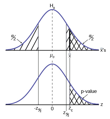
The calculated value of the test in this example and is marked on the bottom graph of the standard normal distribution because it is a Z value. In this case the calculated value is in the tail and thus we cannot accept the null hypothesis, the associated is just too unusually large to believe that it came from the distribution with a mean of with a significance level of .
If we use the p-value decision rule, we need one more step. We need to find in the standard normal table the probability associated with the calculated test statistic, . We then compare that to the associated with our selected level of confidence. In Figure 12 we see that the p-value is less than and therefore we cannot accept the null. We know that the p-value is less than because the area under the p-value is smaller than . It is important to note that two researchers drawing randomly from the same population may find two different P-values from their samples. This occurs because the P-value is calculated as the probability in the tail beyond the sample mean assuming that the null hypothesis is correct. Because the sample means will in all likelihood be different this will create two different P-values. Nevertheless, the conclusions as to the null hypothesis should be different with only the level of probability of .
Here is a systematic way to make a decision of whether you cannot accept or cannot reject a null hypothesis if using the p-value and a preset or preconceived α (the “significance level”). A preset is the probability of a Type I error (rejecting the null hypothesis when the null hypothesis is true). It may or may not be given to you at the beginning of the problem. In any case, the value of α is the decision of the analyst. When you make a decision to reject or not reject , do as follows:
- If
 p-value, cannot accept . The results of the sample data are significant. There is sufficient evidence to conclude that is an incorrect belief and that the alternative hypothesis, , may be correct.
 - If
 p-value, cannot reject . The results of the sample data are not significant. There is not sufficient evidence to conclude that the alternative hypothesis, , may be correct. In this case the status quo stands.
 - When you “cannot reject ,” it does not mean that you should believe that is true. It simply means that the sample data have failed to provide sufficient evidence to cast serious doubt about the truthfulness of . Remember that the null is the status quo, and it takes high probability to overthrow the status quo. This bias in favor of the null hypothesis is what gives rise to the statement “tyranny of the status quo” when discussing hypothesis testing and the scientific method.
Both decision rules will result in the same decision, and it is a matter of preference which one is used.
What is a “P-Value?”
One and Two-Tailed Tests
The discussion with the figures above was based on the null and alternative hypothesis presented in the first figure. This was called a two-tailed test because the alternative hypothesis allowed that the mean could have come from a population which was either larger or smaller than the hypothesized mean in the null hypothesis. This could be seen by the statement of the alternative hypothesis as  , in this example.
It may be that the analyst has no concern about the value being “too” high or “too” low from the hypothesized value. If this is the case, it becomes a one-tailed test, and all of the alpha probability is placed in just one tail and not split into as in the above case of a two-tailed test. Any test of a claim will be a one-tailed test. For example, a car manufacturer claims that their Model 17B provides gas mileage of greater than 25 miles per gallon. The null and alternative hypothesis would be:


The claim would be in the alternative hypothesis. The burden of proof in hypothesis testing is carried in the alternative. This is because failing to reject the null, the status quo, must be accomplished with 90 or 95 percent confidence that it cannot be maintained. Said another way, we want to have only a 5 or 10 percent probability of making a Type I error, rejecting a good null; overthrowing the status quo.
This is a one-tailed test, and all of the alpha probability is placed in just one tail and not split into as in the above case of a two-tailed test.
Figure 13 shows two possible cases and the form of the null and alternative hypothesis that give rise to them.
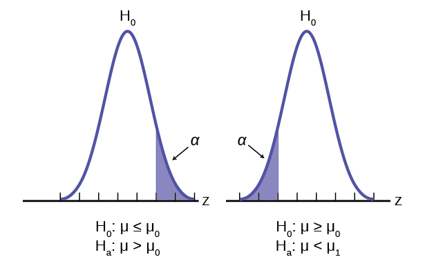
Where is the hypothesized value of the population mean.
| Sample size | Test statistic |
|---|---|
  |
 |
 |
 |
  |
 |

|
|
Effects of Sample Size on Test Statistic
In developing the confidence intervals for the mean from a sample, we found that most often we would not have the population standard deviation, . If the sample size were less than 30, we could simply substitute the point estimate for , the sample standard deviation, s, and use the student’s t-distribution to correct for this lack of information.
When testing hypotheses, we are faced with this same problem and the solution is exactly the same. Namely: If the population standard deviation is unknown, and the sample size is less than 30, substitute s, the point estimate for the population standard deviation, , in the formula for the test statistic and use the student’s t-distribution. All the formulas and figures above are unchanged except for this substitution and changing the Z distribution to the student’s t-distribution on the graph. Remember that the student’s t-distribution can only be computed knowing the proper degrees of freedom for the problem. In this case, the degrees of freedom is computed as before with confidence intervals:  . The calculated t-value is compared to the t-value associated with the pre-set level of confidence required in the test,
  found in the student’s t tables. If we do not know , but the sample size is 30 or more, we simply substitute s for and use the normal distribution.
Table 8 summarizes these rules.
A Systematic Approach for Testing a Hypothesis
A systematic approach to hypothesis testing follows the following steps and in this order. This template will work for all hypotheses that you will ever test.
- Set up the null and alternative hypothesis. This is typically the hardest part of the process. Here the question being asked is reviewed. What parameter is being tested, a mean, a proportion, differences in means, etc. Is this a one-tailed test or two-tailed test?
- Decide the level of significance required for this particular case and determine the critical value. These can be found in the appropriate statistical table. The levels of confidence typical for businesses are 80, 90, 95, 98, and 99. However, the level of significance is a policy decision and should be based upon the risk of making a Type I error, rejecting a good null. Consider the consequences of making a Type I error.
Next, on the basis of the hypotheses and sample size, select the appropriate test statistic and find the relevant critical value: , etc. Drawing the relevant probability distribution and marking the critical value is always big help. Be sure to match the graph with the hypothesis, especially if it is a one-tailed test.
 - Take a sample(s) and calculate the relevant parameters: sample mean, standard deviation, or proportion. Using the formula for the test statistic from above in step 2, now calculate the test statistic for this particular case using the parameters you have just calculated.
- Compare the calculated test statistic and the critical value. Marking these on the graph will give a good visual picture of the situation. There are now only two situations:
- The test statistic is in the tail: Cannot Accept the null, the probability that this sample mean (proportion) came from the hypothesized distribution is too small to believe that it is the real home of these sample data.
- The test statistic is not in the tail: Cannot Reject the null, the sample data are compatible with the hypothesized population parameter.
- Reach a conclusion. It is best to articulate the conclusion two different ways. First a formal statistical conclusion such as “With a 5 % level of significance we cannot accept the null hypotheses that the population mean is equal to XX (units of measurement)”. The second statement of the conclusion is less formal and states the action, or lack of action, required. If the formal conclusion was that above, then the informal one might be, “The machine is broken, and we need to shut it down and call for repairs.”
All hypotheses tested will go through this same process. The only changes are the relevant formulas and those are determined by the hypothesis required to answer the original question.
Hypothesis Testing: One Sample Z Test of the Mean (Critical Value Approach)
Hypothesis Testing: t Test for the Mean (Critical Value Approach)
Hypothesis Testing: 1 Sample Z Test of the Mean (Confidence Interval Approach)
Hypothesis Testing: 1 Sample Z Test for Mean (P-Value Approach)
Hypothesis Test for Proportions
Just as there were confidence intervals for proportions, or more formally, the population parameter p of the binomial distribution, there is the ability to test hypotheses concerning p.
The population parameter for the binomial is p. The estimated value (point estimate) for p is p’ where  is the number of successes in the sample and n is the sample size.
When you perform a hypothesis test of a population proportion p, you take a simple random sample from the population. The conditions for a binomial distribution must be met, which are: there are a certain number n of independent trials meaning random sampling, the outcomes of any trial are binary, success or failure, and each trial has the same probability of a success p. The shape of the binomial distribution needs to be similar to the shape of the normal distribution. To ensure this, the quantities np’ and nq’ must both be greater than five  . In this case the binomial distribution of a sample (estimated) proportion can be approximated by the normal distribution with
  . Remember that . There is no distribution that can correct for this small sample bias and thus if these conditions are not met, we simply cannot test the hypothesis with the data available at that time. We met this condition when we first were estimating confidence intervals for p.
Again, we begin with the standardizing formula modified because this is the distribution of a binomial.

Substituting  , the hypothesized value of p, we have:

This is the test statistic for testing hypothesized values of p, where the null and alternative hypotheses take one of the following forms:
| Two-tailed test | One-tailed test | One-tailed test |
|---|---|---|
 |
 |
 |
 |
 |
 |
The decision rule stated above applies here also: if the calculated value of shows that the sample proportion is “too many” standard deviations from the hypothesized proportion, the null hypothesis cannot be accepted. The decision as to what is “too many” is pre-determined by the analyst depending on the level of significance required in the test.
Hypothesis Testing: 1 Proportion using the Critical Value Approach
Hypothesis Testing with Two Samples
Studies often compare two groups. For example, researchers are interested in the effect aspirin has in preventing heart attacks. Over the last few years, newspapers and magazines have reported various aspirin studies involving two groups. Typically, one group is given aspirin and the other group is given a placebo. Then, the heart attack rate is studied over several years.
There are other situations that deal with the comparison of two groups. For example, studies compare various diet and exercise programs. Politicians compare the proportion of individuals from different income brackets who might vote for them. Students are interested in whether SAT or GRE preparatory courses really help raise their scores. Many business applications require comparing two groups. It may be the investment returns of two different investment strategies, or the differences in production efficiency of different management styles.
To compare two means or two proportions, you work with two groups. The groups are classified either as independent or matched pairs. Independent groups consist of two samples that are independent, that is, sample values selected from one population are not related in any way to sample values selected from the other population. Matched pairs consist of two samples that are dependent. The parameter tested using matched pairs is the population mean. The parameters tested using independent groups are either population means or population proportions of each group.
Comparing Two Independent Population Means
The comparison of two independent population means is very common and provides a way to test the hypothesis that the two groups differ from each other. Is the night shift less productive than the day shift, are the rates of return from fixed asset investments different from those from common stock investments, and so on? An observed difference between two sample means depends on both the means and the sample standard deviations. Very different means can occur by chance if there is great variation among the individual samples. The test statistic will have to account for this fact. The test comparing two independent population means with unknown and possibly unequal population standard deviations is called the Aspin-Welch t-test. The degrees of freedom formula we will see later was developed by Aspin-Welch.
When we developed the hypothesis test for the mean and proportions, we began with the Central Limit Theorem. We recognized that a sample mean came from a distribution of sample means, and sample proportions came from the sampling distribution of sample proportions. This made our sample parameters, the sample means and sample proportions, into random variables. It was important for us to know the distribution that these random variables came from. The Central Limit Theorem gave us the answer: the normal distribution. Our Z and t statistics came from this theorem. This provided us with the solution to our question of how to measure the probability that a sample mean came from a distribution with a particular hypothesized value of the mean or proportion. In both cases that was the question: what is the probability that the mean (or proportion) from our sample data came from a population distribution with the hypothesized value we are interested in?
Now we are interested in whether or not two samples have the same mean. Our question has not changed: Do these two samples come from the same population distribution? We recognize that we have two sample means, one from each set of data, and thus we have two random variables coming from two unknown distributions. To solve the problem, we create a new random variable, the difference between the sample means. This new random variable also has a distribution and, again, the Central Limit Theorem tells us that this new distribution is normally distributed, regardless of the underlying distributions of the original data. A graph may help to understand this concept.
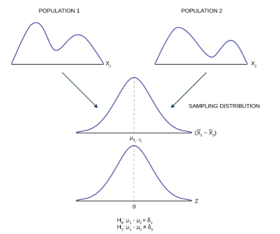
Pictured in Figure 14 are two distributions of data,  , with unknown means and standard deviations. The second panel shows the sampling distribution of the newly created random variable
  . This distribution is the theoretical distribution of many samples means from population 1 minus sample means from population 2. The Central Limit Theorem tells us that this theoretical sampling distribution of differences in sample means is normally distributed, regardless of the distribution of the actual population data shown in the top panel. Because the sampling distribution is normally distributed, we can develop a standardizing formula and calculate probabilities from the standard normal distribution in the bottom panel, the Z distribution.
The Central Limit Theorem, as before, provides us with the standard deviation of the sampling distribution, and further, that the expected value of the mean of the distribution of differences in sample means is equal to the differences in the population means. Mathematically this can be stated:

Because we do not know the population standard deviations, we estimate them using the two sample standard deviations from our independent samples. For the hypothesis test, we calculate the estimated standard deviation, or standard error, of the difference in sample means,  .
.
The standard error is:

We remember that substituting the sample variance for the population variance when we did not have the population variance was the technique we used when building the confidence interval and the test statistic for the test of hypothesis for a single mean back in Confidence Intervals and Hypothesis Testing with One Sample. The test statistic (t-score) is calculated as follows:

Where:
 , the sample standard deviations, are estimates of
  , respectively
- are the unknown population standard deviations
 are the sample means.
  are the unknown population means.
The number of degrees of freedom (df) requires a somewhat complicated calculation. The df are not always a whole number. The test statistic above is approximated by the Student’s t-distribution with df as follows:

When both sample sizes  are 30 or larger, the Student’s t approximation is very good. If each sample has more than 30 observations, then the degrees of freedom can be calculation as
  .
.
The format of the sampling distribution, differences in sample means, specifies that the format of the null and alternative hypothesis is:


Where  is the hypothesized difference between the two means. If the question is simply “is there any difference between the means?” then
  and the null and alternative hypotheses becomes:


An example of when might not be zero is when the comparison of the two groups requires a specific difference for the decision to be meaningful. Imagine that you are making a capital investment. You are considering changing from your current model machine to another. You measure the productivity of your machines by the speed they produce the product. It may be that a contender to replace the old model is faster in terms of product throughout but is also more expensive. The second machine may also have more maintenance costs, setup costs, etc. The null hypothesis would be set up so that the new machine would have to be better than the old one by enough to cover these extra costs in terms of speed and cost of production. This form of the null and alternative hypothesis shows how valuable this particular hypothesis test can be. For most of our work we will be testing simple hypotheses asking if there is any difference between the two-distribution means.
Hypothesis Testing – Two Population Means
Two Population Means, One Tail Test
Two Population Means, Two Tail Test
Check Your Understanding: Hypothesis Testing (Two Population Means)
Cohen’s Standards for Small, Medium, and Large Effect Sizes
Cohen's d is a measure of “effect size” based on the differences between two means. Cohen’s d, named for United States statistician Jacob Cohen, measures the relative strength of the differences between the means of two populations based on sample data. The calculated value of effect size is then compared to Cohen’s standards of small, medium, and large effect sizes.
| Size of effect | d |
|---|---|
| Small | 0.2 |
| Medium | 0.5 |
| Large | 0.8 |
Cohen’s d is the measure of the difference between two means divided by the pooled standard deviation:

It is important to note that Cohen’s d does not provide a level of confidence as to the magnitude of the size of the effect comparable to the other tests of hypothesis we have studied. The sizes of the effects are simply indicative.
Effect Size for a Significant Difference of Two Sample Means
Test for Differences in Means: Assuming Equal Population Variances
Typically, we can never expect to know any of the population parameters, mean, proportion, or standard deviation. When testing hypotheses concerning differences in means we are faced with the difficulty of two unknown variances that play a critical role in the test statistic. We have been substituting the sample variances just as we did when testing hypotheses for a single mean. And as we did before, we used a Student’s t to compensate for this lack of information on the population variance. There may be situations, however, when we do not know the population variances, but we can assume that the two populations have the same variance. If this is true, then the pooled sample variance will be smaller than the individual sample variances. This will give more precise estimates and reduce the probability of discarding a good null. The null and alternative hypotheses remain the same, but the test statistic changes to:

Where  is the pooled variance given by the formula:

Example: A drug trial is attempted using a real drug and a pill made of just sugar. 18 people are given the real drug in hopes of increasing the production of endorphins. The increase in endorphins is found to be on average 8 micrograms per person, and the sample standard deviation is 5.4 micrograms. 11 people are given the sugar pill, and their average endorphin increase is 4 micrograms with a standard deviation of 2.4. From previous research on endorphins, it is determined that it can be assumed that the variances within the two samples can be assumed to be the same. Test at 5% to see if the population mean for the real drug had a significantly greater impact on the endorphins than the population mean with the sugar pill.
Solution:
First, we begin by designating one of the two groups Group 1 and the other Group 2. This will be needed to keep track of the null and alternative hypotheses. Let us set Group 1 as those who received the actual new medicine being tested and therefore Group 2 is those who received the sugar pill. We can now set up the null and alternative hypothesis as:


This is set up as a one-tailed test with the claim in the alternative hypothesis that the medicine will produce more endorphins than the sugar pill. We now calculate the test statistic which requires us to calculate the pooled variance, using the formula above.

 , allows us to compare the test statistic and the critical value.

The test statistic is clearly in the tail, 2.31 is larger than the critical value of 1.703, and therefore we cannot maintain the null hypothesis. Thus, we conclude that there is significant evidence at the 95% level of confidence that the new medicine produces the effect desired.
Two Population Means with Known Standard Deviations
Even though this situation is not likely (knowing the population standard deviations is very unlikely), the following example illustrates hypothesis testing for independent means with known population standard deviations. The sampling distribution for the difference between the means is normal in accordance with the central limit theorem. The random variable is . The normal distribution has the following format:
The standard deviation is:

The test statistic (z-score) is:

Two Population Means, One Tail Test
Two Population Means, Two Tail Test
Check Your Understanding: Two Population Means
Matched or Paired Samples
In most cases of economic or business data we have little or no control over the process of how the data are gathered. In this sense the data are not the result of a planned controlled experiment. In some cases, however, we can develop data that are part of a controlled experiment. This situation occurs frequently in quality control situations. Imagine that the production rates of two machines built to the same design, but at different manufacturing plants, are being tested for differences in some production metric such as speed of output or meeting some production specification such as strength of the product. The test is the same in format to what we have been testing, but here we can have matched pairs for which we can test if differences exist. Each observation has its matched pair against which differences are calculated. First, the differences in the metric to be tested between the two lists of observations must be calculated, and this is typically labeled with the letter “d.” Then, the average of these matched differences,  is calculated as is its standard deviation,
  . We expect that the standard deviation of the differences of the matched pairs will be smaller than unmatched pairs because presumably fewer differences should exist because of the correlation between the two groups.
When using a hypothesis test for matched or paired samples, the following characteristics may be present:
-
-
- Simple random sampling is used.
- Sample sizes are often small.
- Two measurements (samples) are drawn from the same pair of individuals or objects.
- Differences are calculated from the matched or paired samples.
- The differences form the sample that is used for the hypothesis test.
- Either the matched pairs have differences that come from a population that is normal or the number of differences is sufficiently large so that distribution of the sample mean of differences is approximately normal.
-
In a hypothesis test for matched or paired samples, subjects are matched in pairs and differences are calculated. The differences are the data. The population mean for the differences,  , is then tested using a Student’s t-test for a single population mean with degrees of freedom, where n is the number of differences, that is, the number of pairs not the number of observations.
The null and alternative hypotheses for this test are:


The test statistic is:

Two Population Means, One Tail Test, Matched Sample
Two Population Means, One Tail test, Matched Sample (Hypothesized Test Different from Zero)
Matched Sample, Two Tail Test
Check Your Understanding: Matched Sample, Two Tail Test
Comparing Two Independent Population Proportions
When conducting a hypothesis test that compares two independent population proportions, the following characteristics should be present:
-
-
- The two independent samples are random samples are independent.
- The number of successes is at least five, and the number of failures is at least five, for each of the samples.
- Growing literature states that the population must be at least ten or even perhaps 20 times the size of the sample. This keeps each population from being over-sampled and causing biased results.
-
Comparing two proportions, like comparing two means, is common. If two estimated proportions are different, it may be due to a difference in the populations or it may be due to chance in the sampling. A hypothesis test can help determine if a difference in the estimated proportions reflects a difference in the two population proportions.
Like the case of differences in sample means, we construct a sampling distribution for differences in sample proportions:  where
where  are the sample proportions for the two sets of data in question.
  are the number of successes in each sample group respectively, and
  are the respective sample sizes from the two groups. Again, we go the Central Limit Theorem to find the distribution of this sampling distribution for the differences in sample proportions. And again, we find that this sampling distribution, like the one’s past, are normally distributed as proved by the Central Limit Theorem, as see in Figure 15.
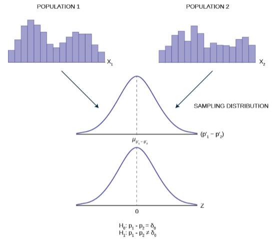
Generally, the null hypothesis allows for the test of a difference of a particular value, , just as we did for the case of difference in means.


Most common, however, is the test that the two proportions are the same. That is,


To conduct the test, we use a pooled proportion,  .
.
The pooled proportion is calculated as follows:

The test statistic (z-score) is:

Where is the hypothesized differences between the two proportions and is the pooled variance from the formula above.
Two Population Proportions, One Tail Test
Two Population Proportion, Two Tail Test
Check Your Understanding: Comparing Two Independent Population Proportions
The Chi-Square Distribution
Have you ever wondered if lottery winning numbers were evenly distributed or if some numbers occurred with a greater frequency? How about if the types of movies people preferred were different across different age groups? What about if a coffee machine was dispensing approximately the same amount of coffee each time? You could answer these questions by conducting a hypothesis test.
You will now study a new distribution, one that is used to determine the answers to such questions. This distribution is called the chi-square distribution.
In this section, you will learn the three major applications of the chi-square distribution:
-
- The test of a single variance, which tests variability, such as in the coffee example
- The goodness-of-fit test, which determines if data fit a particular distribution, such as in the lottery example
- the test of independence, which determines if events are independent, such as in the movie example
Facts About the Chi-Square Distribution
The notation for the chi-square distribution is:

Where  degrees of freedom which depends on how chi-square is being used. (If you want to practice calculating chi-square probabilities then use
  . The degrees of freedom for the three major uses are each calculated differently.)
For the  distribution, the population mean is
  and the population standard deviation is
  .
.
The random variable is shown as .
The random variable for a chi-square distribution with k degrees of freedom is the sum of k independent, squared standard normal variables.

-
-
- The curve is nonsymmetrical and skewed to the right.
- There is a different chi-square curve for each df.
-
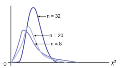
3. The test statistic for any test is always greater than or equal to zero.
4. When  , the chi-square curve approximates the normal distribution. For
  the mean,
  and the standard deviation,
  . Therefore,
  , approximately.
5. The mean, is located just to the right of the peak.
Test of a Single Variance
Thus far our interest has been exclusively on the population parameter or it is counterpart in the binomial, p. Surely the mean of a population is the most critical piece of information to have, but in some cases, we are interested in the variability of the outcomes of some distribution. In almost all production processes quality is measured not only by how closely the machine matches the target, but also the variability of the process. If one were filling bags with potato chips not only would there be interest in the average weight of the bag, but also how much variation there was in the weights. No one wants to be assured that the average weight is accurate when their bag has no chips. Electricity voltage may meet some average level, but great variability, spikes, can cause serious damage to electrical machines, especially computers. I would not only like to have a high mean grade in my classes, but also low variation about this mean. In short, statistical tests concerning the variance of a distribution have great value and many applications.
A test of a single variance assumes that the underlying distribution is normal. The null and alternative hypotheses are stated in terms of the population variance. The test statistic is:

Where:
 the total number of observations in the sample data
 sample variance
 hypothesized value of the population variance

You may think of s as the random variable in this test. The number of degrees of freedom is . A test of a single variance may be right-tailed, left-tailed, or two-tailed. The example below will show you how to set up the null and alternative hypotheses. The null and alternative hypotheses contain statements about the population variance.
Example: Math instructors are not only interested in how their students do on exams, on average, but how the exam scores vary. To many instructors, the variance (or standard deviation) may be more important than the average.
Suppose a math instructor believes that the standard deviation for his final exam is five points. One of his best students thinks otherwise. The student claims that the standard deviation is more than five points. If the student were to conduct a hypothesis test, what would the null and alternative hypotheses be?
Solution: Even though we are given the population standard deviation, we can set up the test using the population variance as follows:


Single Population Variances, One-Tail Test
Check Your Understanding: Test of a Single Variance
Goodness-Of-Fit Test
In this type of hypothesis test, you determine whether the data “fit” a particular distribution or not. For example, you may suspect your unknown data fit a binomial distribution. You use a chi-square test (meaning the distribution for the hypothesis test is chi-square) to determine if there is a fit or not. The null and the alternative hypotheses for this test may be written in sentences or may be stated as equations or inequalities.
The test statistic for a goodness-of -fit test is:

Where:
- O = observed values (data)
- E = expected values (from theory)
- k = the number of different data cells or categories
The observed values are the data values, and the expected values are the values you would expect to get it the null hypothesis were true. There are n terms of the form  .
.
The number of degrees of freedom is  .
.
The goodness-of-fit test is almost always right-tailed. If the observed values and the corresponding expected values are not close to each other, then the test statistic can get very large and will be way out in the right tail of the chi-square curve.
Note: The number of expected values inside each cell needs to be at least five in order to use this test.
Chi-Square Statistic for Hypothesis Testing
Chi-Square Goodness-of-Fit Example
Check Your Understanding: Goodness-of-Fit Test
Test of Independence
Tests of independence involve using a contingency table of observed (data) values.
The test statistic of a test of independence is similar to that of a goodness-of-fit test:

Where:
- O = observed values
- E = expected values
- i = the number of rows in the table
- j = the number of columns in the table
There are 
A test of independence determines whether two factors are independent or not.
Note: The expected value inside each cell needs to be at least five in order for you to use this test.
The test of independence is always right tailed because of the calculation of the test statistic. If the expected and observed values are not close together, then the test statistic is very large and way out in the right tail of the chi-square curve, as it is in a goodness-of-fit.
The number of degrees of freedom for the test of independence is:

The following formula calculates the expected number (E):

Simple Explanation of Chi-Squared
Chi-Square Test for Association (independence)
Check Your Understanding: Test of Independence
Test for Homogeneity
The goodness-of-fit test can be used to decide whether a population fits a given distribution, but it will not suffice to decide whether two populations follow the same unknown distribution. A different test, called the test of homogeneity, can be used to draw a conclusion about whether two populations have the same distribution. To calculate the test statistic for a test for homogeneity, follow the same procedure as with the test of independence.
Note: The expected value inside each cell needs to be at least five in order for you to use this test.
Hypotheses
: The distribution of the two populations is the same.
 The distributions of the two population are not the same.
Test Statistic
Use a test statistic. It is computed in the same way as the test for independence.
Degrees of Freedom (df)

Requirements
All values in the table must be greater than or equal to five
Common uses
Comparing two populations. For example: men vs. women, before vs. after, east vs. west. The variable is categorical with more than two possible response values.
Introduction to the Chi-Square Test for Homogeneity
Check Your Understanding: Test for Homogeneity
Comparison of the Chi-Square Tests
Above the test statistic was used in three different circumstances. The following bulleted list is a summary of which test is the appropriate one to use in different circumstances.
Goodness-of-fit: Use the goodness-of-fit test to decide whether a population with an unknown distribution “fits” a known distribution. In this case there will be a single qualitative survey question or a single outcome of an experiment from a single population. Goodness-of-Fit is typically used to see if the population is uniform (all outcomes occur with equal frequency), the population is normal, or the population is the same as another population with a known distribution. The null and alternative hypotheses are:
The population fits given distribution
The population does not fit the given distribution
Independence: Use the test for independence to decide whether two variables (factors) are independent or dependent. In this case there will be two qualitative survey questions or experiments and a contingency table will be constructed. The goal is to see if the two variables are unrelated (independent) or related (dependent). The null and alternative hypotheses are:
The two variables (factors) are independent
The two variables (factors) are dependent
Homogeneity: Use the test for homogeneity to decide if two populations with unknown distributions have the same distribution as each other. In this case there will be a single qualitative survey question or experiment given to two different populations. The null and alternative hypotheses are:
The two populations follow the same distribution
: The two populations have different distributions
F Distribution and One-Way ANOVA
Many statistical applications in psychology, social science, business administration, and the natural sciences involve several groups. For example, an environmentalist is interested in knowing if the average amount of pollution varies in several bodies of water. A sociologist is interested in knowing if the amount of income a person earns varies according to his or her upbringing. A consumer looking for a new car might compared the average gas mileage of several models.
For hypothesis tests comparing averages among more than two groups, statisticians have developed a method called “Analysis of Variance” (abbreviated ANOVA). In this chapter, you will study the simplest form of ANOVA called single factor or one-way ANOVA. You will also study the F distribution, used for one-way ANOVA, and the test for differences between two variances. This is just a very brief overview of one-way ANOVA. One-Way ANOVA, as it is presented here, relies heavily on a calculator or computer.
Test of Two Variances
This chapter introduces a new probability density function, the F distribution. This distribution is used for many applications including ANOVA and for testing equality across multiple means. We begin with the F distribution and the test of hypothesis of differences in variances. It is often desirable to compare two variances rather than two averages. For instance, college administrators would like two college professors grading exams to have the same variation in their grading. In order for a lid to fit a container, the variation in the lid and the container should be approximately the same. A supermarket might be interested in the variability of check-out times for two checkers. In finance, the variance is a measure of risk and thus an interesting question would be to test the hypothesis that two different investment portfolios have the same variance, the volatility.
In order to perform a F test of two variances, it is important that the following are true:
-
-
- The populations from which the two samples are drawn are approximately normally distributed.
- The two populations are independent of each other.
-
Unlike most other hypothesis tests in this Module, the F test for equality of two variances is very sensitive to deviations from normality. If the two distributions are not normal, or close, the test can give a biased result for the test statistic.
Suppose we sample randomly from two independent normal populations. Let  be the unknown population variances and
  be the sample variances. Let the sample sizes be . Since we are interested in comparing the two sample variances, we use the F ratio:
![\boldsymbol{F}=\frac{\left[\frac{s_1^2}{\sigma_1^2}\right]}{\left[\frac{s_2^2}{\sigma_2^2}\right]}](https://uta.pressbooks.pub/app/uploads/quicklatex/quicklatex.com-a4cbd7aa37d0937b0f795ee972b65c05_l3.png "Rendered by QuickLaTeX.com")
F has the distribution 
Where  are the degrees of freedom for the numerator and
  are the degrees of freedom for the denominator.
If the null hypothesis is  , then the F Ratio, test statistic, becomes
![F_c=\frac{\left[\frac{s_1^2}{\sigma_1^2}\right]}{\left[\frac{s_2^2}{\sigma_2^2}\right]}=\frac{s_1^2}{s_2^2}](https://uta.pressbooks.pub/app/uploads/quicklatex/quicklatex.com-0bd03e56b454884205df0b9800a8511b_l3.png "Rendered by QuickLaTeX.com")
The various forms of the hypotheses tested are:
| Two-Tailed Test | One-Tailed Test | One-Tailed Test |
|---|---|---|
 |
 |
 |
 |
 |
 |
A more general form of the null and alternative hypothesis for a two tailed test would be:


Where if  it is a simple test of the hypothesis that the two variances are equal. This form of the hypothesis does have the benefit of allowing for tests that are more than for simple differences and can accommodate tests for specific differences as we did for differences in means and differences in proportions. This form of the hypothesis also shows the relationship between the F distribution and the : the F is a ratio of two chi squared distributions a distribution we saw in the last chapter. This is helpful in determining the degrees of freedom of the resultant F distribution.
If the two populations have equal variances, then are close in value and the test statistic,  is close to one. But if the two population variances are very different, tend to be very different, too. Choosing
  as the larger sample variance causes the ratio
  to be greater than one. If are far apart, then is a large number.
Therefore, if F is close to one, the evidence favors the null hypothesis (the two population variances are equal). But if F is much larger than one, then the evidence is against the null hypothesis. In essence, we are asking if the calculated F statistic, test statistic, is significantly different from one.
To determine the critical points, we have to find  . This F table has values for various levels of significance from 0.1 to 0.001 designated as “p” in the first column. To find the critical value choose the desired significance level and follow down and across to find the critical value at the intersection of the two different degrees of freedom. The F distribution has two different degrees of freedom, one associated with the numerator,
  , and one associated with the denominator,
  and to complicate matters, the F distribution is not symmetrical and changes the degree of skewness as the degrees of freedom of change. The degrees of freedom in the numerator is
  is the sample size for group 1, and the degrees of freedom in the denominator is , where
  is the sample size for group 2. will give the critical value on the upper end of the F distribution.
To find the critical value for the lower end of the distribution, reverse the degrees of freedom and divide the F-value from the table into one.
- Upper tail critical value:
- Lower tail critical value:

When the calculated value of F is between the critical values, not in the tail, we cannot reject the null hypothesis that the two variances came from a population with the same variance. If the calculated F-value is in either tail we cannot accept the null hypothesis just as we have been doing for all of the previous tests of hypothesis.
An alternative way of finding the critical values of the F distribution makes the use of the F-table easier. We note in the F-table that all the values of F are greater than one therefore the critical F value for the left-hand tail will always be less than one because to find the critical value on the left tail we divide an F value into the number one as shown above. We also note that if the sample variance in the numerator of the test statistic is larger than the sample variance in the denominator, the resulting F value will be greater than one. The shorthand method for this test is thus to be sure that the larger of the two sample variances is placed in the numerator to calculate the test statistic. This will mean that only the right-hand tail critical value will have to be found in the F-table.
Hypothesis Test Two Population Variances
Check Your Understanding: F Distribution
One-Way ANOVA
The purpose of a one-way ANOVA test is to determine the existence of a statistically significant difference among several group means. The test actually uses variances to help determine if the means are equal or not. In order to perform a one-way ANOVA test, there are five basic assumptions to be fulfilled:
-
-
- Each population from which a sample is taken is assumed to be normal.
- All samples are randomly selected and independent.
- The populations are assumed to have equal standard deviations (or variances).
- The factor is a categorical variable.
- The response is a numerical variable.
-
The Null and Alternative Hypotheses
The null hypothesis is simply that all the group population means are the same. The alternative hypothesis is that at least one pair of means is different. For example, if there are k groups:

At least two of the group means  are not equal. That is,
  .
.
The graphs, a set of box plots representing the distribution of values with the group means indicated by a horizontal line through the box, help in the understanding of the hypothesis test. In the first graph (red box plots),  and the three populations have the same distribution if the null hypothesis is true. The variance of the combined data is approximately the same as the variance of the populations.
If the null hypothesis is false, then the variance of the combined data is larger which is caused by the different means as shown in the second graph (green box plots).
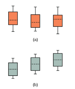 is true. All means are the same; the differences are due to random variation. (b) is not true. All means are not the same; the differences are too large to be due to random variation.
 ANOVA
The F Distribution and the F-Ratio
The distribution used for the hypothesis test is a new one. It is called the F distribution, invented by George Snedecor but named in honor of Sir Ronald Fisher, an English statistician. The F statistic is a ratio (a fraction). There are two sets of degrees of freedom: one for the numerator and one for the denominator.
For example, if F follows an F distribution and the number of degrees of freedom for the numerator is four, and the number of degrees of freedom for the denominator is ten, then  .
.
To calculate the F ratio, two estimates of the variance are made.
-
-
- Variance between samples: An estimate of
 that is the variance of the sample means multiplied by n (when the sample sizes are the same). If the samples are different sizes, the variances between samples is weighted to account for the different sample sizes. The variances is also called variance due to treatment or explained variation.
 - Variance within samples: An estimate of that is the average of the sample variances (also known as a pooled variance). When the sample sizes are different, the variance within samples is weighted. The variance is also called the variation due to error or unexplained variation.
- Variance between samples: An estimate of
-
 the sum of squares that represents the variation among the different samples
 the sum of squares that represents the variation within samples that is due to chance.
To find a “sum of squares” means to add together squared quantities that, in some cases, may be weighted.
MS means “mean square.”  is the variance between groups, and
  is the variance within groups.
Calculation of Sum of Squares and Mean Square
- k = the number of different groups
 group
group group
group- n = total number of all the values combined (total sample size:
 )
) - x = one value:

- Sum of squares of all values from every group combined:

- Between group variability:

- Total sum of squares:

- Explains variation: sum of squares representing variation among the different samples:

- Unexplained variation: sum of squares represent variation within samples due to change:

- d f’s for different groups (d f’s for the numerator):

- Equation for errors within samples (d f’s for the denominator):

- Mean square (variance estimate) explained by the different groups:

- Mean square (variance estimate) that is due to chance (unexplained):

 can be written as follows:


The one-way ANOVA test depends on the fact that can be influenced by population differences among means of the several groups. Since  compares values of each group to its own group mean, the fact that group means might be different does not affect .
The null hypothesis says that all groups are samples from populations having the same normal distribution. The alternate hypothesis says that at least two of the sample groups come from populations with different normal distributions. If the null hypothesis is true, and should both estimate the same value.
Note: The null hypothesis says that all the group population means are equal. The hypothesis of equal means implies that the populations have the same normal distribution, because it is assumed that the populations are normal and that they have equal variances.
F-Ration or F Statistic

If estimate the same value (following the belief that is true), then the F-ratio should be approximately equal to one. Mostly, just sampling errors would contribute to variations away from one. As it turns out, consists of the population variance plus a variance produced form the differences between the samples. is an estimate of the population variance. Since variances are always positive, if the null hypothesis is false, will generally be larger than . Then the F-ratio will be larger than one. However, if the population effect is small, it is not unlikely that will be larger in a given sample.
The foregoing calculations were done with groups of different sizes. If the groups are the same size, the calculations simplify somewhat, and the F-ratio can be written as:
F-Ratio Formula when the groups are the same size

Where:
- n = the sample size


 the mean of the sample variances (pooled variance)
 the variance of the sample means.
Data are typically put into a table for easy viewing. One-Way ANOVA results are often displayed is this manner by computer software.
| Source of variation | Sum of squares (SS) | Degrees of freedom (df) | Mean square (MS) | F |
|---|---|---|---|---|
| Factor (Between) | SS(Factor) | k – 1 | MS(Factor) = |
F =  |
| Error (Within) | SS(Error) | n – k | MS(Error) =  |
|
| Total | SS(Total) | n – 1 |
Example: Three different diet plans are to be tested for mean weight loss. The entries in the table are the weight losses for the different plans. The one-way ANOVA results are shown in Table 13.
Plan 1:  |
Plan 2:  |
Plan 3:  |
|---|---|---|
| 5 | 3.5 | 8 |
| 4.5 | 7 | 4 |
| 4 | 3.5 | |
| 3 | 4.5 |

Following are the calculations needed to fill in the one-way ANOVA table. The table is used to conduct a hypothesis test.
![S S_{\text {between }}=\sum\left[\frac{\left(s_j\right)^2}{n_j}\right]-\frac{\left(\sum s_j\right)^2}{n}](https://uta.pressbooks.pub/app/uploads/quicklatex/quicklatex.com-6633d262bf3583714fecc2698c03defc_l3.png "Rendered by QuickLaTeX.com")

Where 


| Source of variation | Sum of squares (SS) | Degrees of freedom (df) | Mean square (MS) | F |
|---|---|---|---|---|
| Factor (Between) |
SS(Factor) =SS(Between) = 2.2458 |
k – 1 = 3 groups – 1 = 2 |
MS(Factor) = SS(Factor)/(k – 1) = 2.2458/2 = 1.1229 |
F = MS(Factor)/MS(Error) = 1.1229/2.9792 = 0.3769 |
| Error (Within) |
SS(Error) = SS(Within) = 20.8542 |
n – k = 10 total data – 3 groups = 7 |
MS (Error) = SS(Error)/(n – k) = 20.8542/7 = 2.9792 |
|
| Total | SS(Total) = 2.2458 + 20.8542 = 23.1 |
n – 1 = 10 total data – 1 = 9 |
The one-way ANOVA hypothesis test is always right-tailed because larger F-values are way out in the right tail of the F-distribution and tend to make us reject .
Notation
The notation for the F distribution is 
Where 
The mean for the F distribution is 
Calculating SST (total sum of squares)
Calculating 
Hypothesis Test with F-Statistic
Check Your Understanding: The F Distribution and the F-Ratio
Facts About the F Distribution
-
-
- The curve is not symmetrical but skewed to the right.
- There is a different curve for each set of degrees of freedom.
- The F statistic is greater than or equal to zero.
- As the degrees of freedom for the numerator and for the denominator get larger, the curve approximates the normal as can be seen in Figure 18. Remember that the F cannot ever be less than zero, so the distribution does not have a tail that goes to infinity on the left as the normal distribution does.
- Other uses for the F distribution include comparing two variances and two-way Analysis of Variances. Two-Way Analysis is beyond the scope of this section.
-
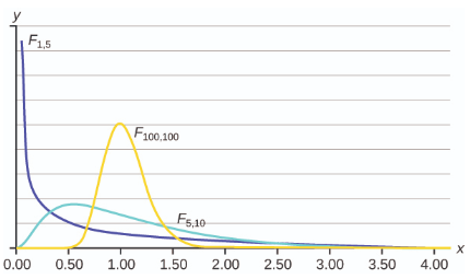
Compute and Interpret Simple Linear Regression Between Two Variables
Linear Regression and Correlation
Professionals often want to know how two or more numeric variables are related. For example, is there a relationship between the grade on the second math exam a student takes and the grade on the final exam? If there is a relationship, what is the relationship and how strong is it?
This example may or may not be tied to a model, meaning that some theory suggested that a relationship exists. This link between a cause and an effect is the foundation of the scientific method and is the core of how we determine what we believe about how the world works. Beginning with a theory and developing a model of the theoretical relationship should result in a prediction, what we have called a hypothesis earlier. Now the hypothesis concerns a full set of relationships.
The foundation of all model building is perhaps the arrogant statement that we know what caused the result we see. This is embodied in the simple mathematical statement of the functional form that  . The response, Y, is caused by the stimulus, X. Every model will eventually come to this final place, and it will be here that the theory will live or die. Will the data support this hypothesis? If so, then fine, we shall believe this version of the world until a better theory comes to replace it. This is the process by which we moved from flat earth to round earth, from earth-center solar system to sun-center solar system, and on and on.
In this section we will begin with correlation, the investigation of relationships among variables that may or may not be founded on a cause-and-effect model. The variables simply move in the same, or opposite, direction. That is to say, they do not move randomly. Correlation provides a measure of the degree to which this is true. From there we develop a tool to measure cause and effect relationships, regression analysis. We will be able to formulate models and tests to determine if they are statistically sound. If they are found to be so, then we can use them to make predictions: if as a matter of policy, we changed the value of this variable what would happen to this other variable? If we imposed a gasoline tax of 50 cents per gallon how would that effect the carbon emissions, sales of Hummers/Hybrids, use of mass transit, etc.? The ability to provide answers to these types of questions is the value of regression as both a tool to help us understand our world and to make thoughtful policy decisions.
The Correlation Coefficient r
As we begin this section, we note that the type of data we will be working with has changed. Perhaps unnoticed, all the data we have been using is for a single variable. It may be from two samples, but it is still a univariate variable. The type of data described for any model of cause and effect is bivariate data — “bi” for two variables. In reality, statisticians use multivariate data, meaning many variables.
Data can be classified into three broad categories: time series data, cross-section data, and panel data. Time series data measures a single unit of observation; say a person, or a company or a country, as time passes. What are measures will be at least two characteristics, say the person’s income, the quantity of a particular good they buy and the price they paid. This would be three pieces of information in one time period, say 1985. If we followed that person across time we would have those same pieces of information for 1985, 1986, 1987, etc. This would constitute a time series data set.
A second type of data set is for cross-section data. Here the variation is not across time for a single unit of observation, but across units of observation during one point in time. For a particular period of time, we would gather the price paid, amount purchased, and income of many individual people.
A third type of data set is panel data. Here a panel of units of observation is followed across time. If we take our example from above, we might follow 500 people, the unit of observation, through time, ten years, and observe their income, price paid and quantity of the good purchased. If we had 500 people and data for ten years for price, income and quantity purchased we would have 15,000 pieces of information. These types of data sets are very expensive to construct and maintain. They do, however, provide a tremendous amount of information that can be used to answer very important questions. As an example, what is the effect on the labor force participation rate of women as their family of origin, mother and father, age? Or are there differential effects on health outcomes depending upon the age at which a person started smoking? Only panel data can give answers to these and related questions because we must follow multiple people across time.
Beginning with a set of data with two independent variables we ask the question: are these related? One way to visually answer this question is to create a scatter plot of the data. We could not do that before when we were doing descriptive statistics because those data were univariate. Now we have bivariate data so we can plot in two dimensions. Three dimensions are possible on a flat piece of paper but become very hard to fully conceptualize. Of course, more than three dimensions cannot be graphed although the relationships can be measured mathematically.
To provide mathematical precision to the measurement of what we see we use the correlation coefficient. The correlation tells us something about the co-movement of two variables, but nothing about why this movement occurred. Formally, correlation analysis assumes that both variables being analyzed are independent variables. This means that neither one causes the movement in the other. Further, it means that neither variable is dependent on the other, or for that matter, on any other variable. Even with these limitations, correlation analysis can yield some interesting results.
The correlation coefficient,  (pronounced rho), is the mathematical statistic for a population that provides us with a measurement of the strength of a linear relationship between the two variables. For a sample of data, the statistic, r, developed by Karl Pearson in the early 1900s, is an estimate of the population correlation and is defined mathematically as:

OR

Where  are the standard deviations of the two independent variables
  are the sample means of the two variables, and
  are the individual observations of . The correlation coefficient r ranges in value from -1 to 1. The second equivalent formula is often used because it may be computationally easier. As scary as these formulas look, they are really just the ratio of the covariance between the two variables and the product of their two standard deviations. That is to say, it is a measure of relative variances.
In practice all correlation and regression analysis will be provided through computer software designed for these purposes. Anything more than perhaps one-half a dozen observations creates immense computational problems. It was because of this fact that correlation, and even more so, regression, were not widely used research tools until after the advent of “computing machines.” Now the computing power required to analyze data using regression packages is deemed almost trivial by comparison to just a decade ago.
To visualize any linear relationship that may exist review the plot of a scatter diagrams of the standardized data. Figure 19 presents several scatter diagrams and the calculated value of r. In panels (a) and (b) notice that the data generally trend together, (a) upward and (b) downward. Panel (a) is an example of a positive correlation and panel (b) is an example of a negative correlation, or relationship. The sign of the correlation coefficient tells us if the relationship is a positive or negative (inverse) one. If all the values of are on a straight line the correlation coefficient will be either  depending on whether the line has a positive or negative slope and the closer to one or negative one the stronger the relationship between the two variables. BUT ALWAYS REMEMBER THAT THE CORRELATION COEFFICIENT DOES NOT TELL US THE SLOPE.
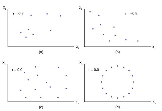
Remember, all the correlation coefficient tells us is whether or not the data are linearly related. In panel (d) the variables obviously have some type of very specific relationship to each other, but the correlation coefficient is zero, indicating no linear relationship exists.
If you suspect a linear relationship between  can measure how strong the linear relationship is.
What the VALUE of r tells us:
- The value of r is always between
 .
. - The size of the correlation r indicates that strength of the linear relationship between . Values of r close to
 indicate a stronger linear relationship between .
 - If
 there is absolutely no linear relationship between (no linear correlation).
 - If
 , there is perfect positive correlation. If
  there is perfect negative correlation. In both these cases, all of the original data points lie on a straight line: ANY straight line no matter what the slope. Of course, in the real world, this will not generally happen.
What the SIGN of r tells us
- A positive value of r means that when
 tends to increase and when
  tend to decrease (positive correlation).
 - A negative value of r means that when tends to decrease and when tends to increase (negative correlation).
Note: Strong correlation does not suggest that  We say, “correlation does not imply causation.”
Bivariate Relationship Linearity, Strength, and Direction
Check Your Understanding: The Correlation Coefficient r
Calculating Correlation Coefficient r
Example: Correlation Coefficient Intuition
Linear Equations
Linear regression to two variables is based on a linear equation with one independent variable. The equation has the form:

Where a and b are constant numbers.
The variable x is the independent variable, and y is the dependent variable. Another way to think about this equation is a statement of cause and effect. The X variable is the cause, and the Y variable is the hypothesized effect. Typically, you choose a value to substitute for the independent variable and then solve for the dependent variable.
The graph of a linear equation of the form is a straight line. Any line that is not vertical can be described by this equation.
Slope and Y-Intercept of a Linear Equation
For the linear equation , b = slope and a = y-intercept. From algebra recall that the slop is a number that described the steepness of a line, and the y-intercept is the y coordinate of the point  where the line crosses the y-axis. From calculus the slope is the first derivative of the function. For a linear function, the slope is
  where we can read the mathematical expression as “the change in
  that results from a change in
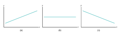 . (a) if b > 0, the line slopes upward to the right. (b) if b=0, the line is horizontal. (c) if b < 0, the line slopes downward to the right.
The Regression Equation
Regression analysis is a statistical technique that can test the hypothesis that a variable is dependent upon one or more other variables. Further, regression analysis can provide an estimate of the magnitude of the impact of a change in one variable on another. This last feature, of course, is all important in predicting future values.
Regression analysis is based upon a functional relationship among variables and further, assumes that the relationship is linear. This linearity assumption is required because, for the most part, the theoretical statistical properties of non-linear estimation are not well worked out yet by the mathematicians and econometricians. This presents us with some difficulties in economic analysis because many of our theoretical models are nonlinear. The marginal cost curve, for example, is decidedly nonlinear as is the total cost function, if we are to believe in the effect of specialization of labor and the Law of Diminishing Marginal Product. There are techniques for overcoming some of these difficulties, exponential and logarithmic transformation of the data for example, but at the outset we must recognize that standard ordinary least squares (OLS) regression analysis will always use a linear function to estimate what might be a nonlinear relationship.
The general linear regression model can be stated by the equation:

Where  is the intercept,
  are the slope between Y and the appropriate
  (pronounced epsilon), is the error term that captures errors in measurement of Y and the effect on Y of any variables missing from the equation that would contribute to explaining variations in Y. This equation is the theoretical population equation and therefore uses Greek letters. The equation we will estimate will have the Roman equivalent symbols. This is parallel to how we kept track of the population parameters and sample parameters before. The symbol for the population mean was and for the sample mean and for the population standard deviation was and for the sample standard deviation was s. The equation that will be estimated with a sample of data for two independent variables will thus be:

As with our earlier work with probability distributions, this model works only if certain assumptions hold. These are that the Y is normally distributed, the errors are also normally distributed with a mean of zero and a constant standard deviation, and that the error terms are independent of the size of X and independent of each other.
Assumptions of the Ordinary Least Squares Regression Model
Each of these assumptions needs a bit more explanation. If one of these assumptions fails to be true, then it will have an effect on the quality of the estimates. Some of the failures of these assumptions can be fixed while others result in estimates that quite simply provide no insight into the questions the model is trying to answer or worse, give biased estimates.
-
- The independent variables,
 , are all measured without error, and are fixed numbers that are independent of the error term. This assumption is saying in effect that Y is deterministic, the result of a fixed component “X” and a random error component “
 .”
.” - The error term is a random variable with a mean of zero and a constant variance. The meaning of this is that the variances of the independent variables are independent of the value of the variable. Consider the relationship between personal income and the quantity of a good purchased as an example of a case where the variance is dependent upon the value of the independent variable, income. It is plausible that as income increases the variation around the amount purchased will also increase simply because of the flexibility provided with higher levels of income. The assumption is for constant variance with respect to the magnitude of the independent variable called homoscedasticity. If the assumption fails, then it is called heteroscedasticity. Figure 21 shows the case of homoscedasticity where all three distributions have the same variance around the predicted value of Y regardless of the magnitude of X.
- Error terms should be normally distributed. This can be seen in Figure 21 by the shape of the distributions placed on the predicted line at the expected value of the relevant value of Y.
- The independent variables are independent of Y but are also assumed to be independent of the other X variables. The model is designed to estimate the effects of independent variables on some dependent variable in accordance with a proposed theory. The case where some or more of the independent variables are correlated is not unusual. There may be no cause and effect relationship among the independent variables, but nevertheless they move together. Take the case of a simple supply curve where quantity supplied is theoretically related to the price of the product and the prices of inputs. There may be multiple inputs that may over time move together from general inflationary pressure. The input prices will therefore violate this assumption of regression analysis. This condition is called multicollinearity.
- The error terms are uncorrelated with each other. This situation arises from an effect on one error term from another error term. While not exclusively a time series problem, it is here that we most often see this case. An X variable in time period one has an effect on the Y variable, but this effect then has an effect in the next time period. This effect gives rise to a relationship among the error terms. This case is called autocorrelation, “self-correlated.” The error terms are now not independent of each other, but rather have their own effect on subsequent error terms.
- The independent variables,
Figure 21 shows the case where the assumptions of the regression model are being satisfied. The estimated line is  . Three values of X are shown. A normal distribution is placed at each point where X equals the estimated line and the associated error at each value of Y. Notice that the three distributions are normally distributed around the point on the line, and further, the variation, variance, around the predicted value is constant indicating homoscedasticity from assumption 2. Figure 21 does not show all the assumptions of the regression model, but it helps visualize these important ones.
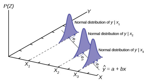
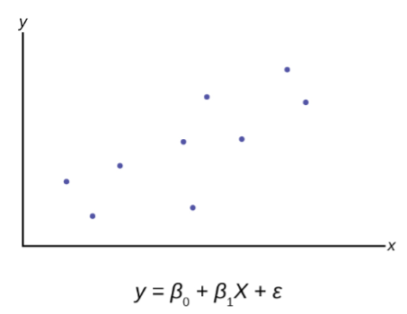
This is the general form that is most often called the multiple regression model. So-called “simple” regression analysis has only one independent (right-hand) variable rather than many independent variables. Simple regression is just a special case of multiple regression. There is some value in beginning with simple regression: it is easy to graph in two dimensions, difficult to graph in three dimensions, and impossible to graph in more than three dimensions. Consequently, our graphs will be for the simple regression case. Figure 22 presents the regression problem in the form of a scatter plot graph of the data set where it is hypothesized that Y is dependent upon the single independent variable X.
The regression problem comes down to determining which straight line would best represent the data in Figure 23. Regression analysis is sometimes called “least squares” analysis because the method of determining which line best “fits” the data is to minimize the sum of the squared residuals of a line put through the data.
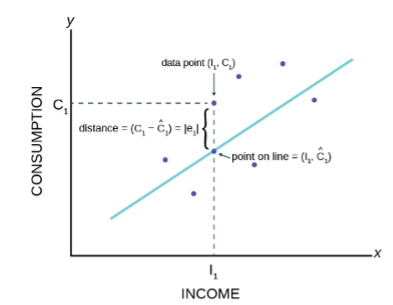
 Estimated Equation:
Figure 23 shows the assumed relationship between consumption and income from macroeconomic theory. Here the data are plotted as a scatter plot and an estimated straight line has been drawn. From this graph we can see an error term,  . Each data point also has an error term. Again, the error term is put into the equation to capture effects on consumption that are not caused by income changes. Such other effects might be a person’s savings or wealth, or periods of unemployment. We will see how by minimizing the sum of these errors we can get an estimate for the slope and intercept of this line.
Consider the graph in Figure 24. The notation has returned to that for the more general model rather than the specific case of the Macroeconomic consumption function in our example.
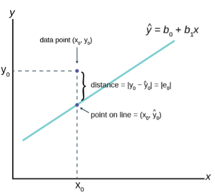
The  is read “y hat” and is the estimated value of y. (In Figure 23
  represents the estimated value of consumption because it is on the estimated line.) It is the value of y obtained using the regression line.
  is not generally equal to y from the data.
The term  is called the “error” or residual. It is not an error in the sense of a mistake. The error term was put into the estimating equation to capture missing variables and error in measurement that may have occurred in the dependent variables. The absolute value of a residual measure the vertical distance between the actual value of y and the estimated value of y. In other words, it measures the vertical distance between the actual data point and the predicted point on the line as can be seen on the graph at point
  .
.
If the observed data point lies above the line, the residual is positive, and the line underestimates the actual data value for y.
If the observed data point lies below the line, the residual is negative, and the line overestimates that actual data value for y.
In the graph,  is the residual for the point shown. Here the point lies above the line, and the residual is positive. For each data point the residuals, or errors, are calculated
  where n is the sample size. Each
  is a vertical distance.
The sum of the errors squared is the term obviously called Sum of Squared Errors (SSE).
Using calculus, you can determine the straight line that has the parameter values of  that minimizes the SSE. When you make the SSE a minimum, you have determined the points that are on the line of best fit. It turns out that the line of best fit has the equation:

The sample means of the x values and the y values are  , respectively. The best fit line always passes through the point
  called the points of means.
The slope b can also be written as:

Where  the standard deviation of the y values and
  the standard deviation of the x values and r is the correlation coefficient between x and y.
These equations are called the Normal Equations and come from another very important mathematical finding called the Gauss-Markov Theorem without which we could not do regression analysis. The Gauss-Markov Theorem tells us that the estimates we get from using the ordinary least squares (OLS) regression method will result in estimates that have some very important properties. In the Gauss-Markov Theorem it was proved that a least squares line is BLUE, which is, Best, Linear, Unbiased, Estimator. Best is the statistical property that an estimator is the one with the minimum variance. Linear refers to the property of the type of line being estimated. An unbiased estimator is one whose estimating function has an expected mean equal to the mean of the population. (You will remember that the expected value  was equal to the population mean in accordance with the Central Limit Theorem. This is exactly the same concept here).
Using the OLS method, we can now find the estimate of the error variance, which is the variance of the squared errors,  . This is sometimes called the standard error of the estimate. (Grammatically this is probably best said as the estimate of the error’s variance). The formula for the estimate of the error variance is:

Where is the predicted value of y and y is the observed value, and thus the term  is the squared errors that are to be minimized to find the estimates of the regression line parameters. This is really just the variance of the error terms and follows our regular variance formula. One important note is that here we are dividing by
  , which is the degrees of freedom. The degrees of freedom of a regression equation will be the number of observations, n, reduced b the number of estimated parameters, which includes the intercept as a parameter.
The variance of the errors is fundamental in testing hypotheses for a regression. It tells us just how “tight” the dispersion is about the line. As we will see shortly, the greater the dispersion about the line, meaning the larger the variance of the errors, the less probable that the hypothesized independent variable will be found to have a significant effect on the dependent variable. In short, the theory being tested will more likely fail if the variance of the error term is high. Upon reflection this should not be a surprise. As we tested hypotheses about a mean we observed that large variances reduced the calculated test statistic and thus it failed to reach the tail of the distribution. In those cases, the null hypotheses could not be rejected. If we cannot reject the null hypothesis in a regression problem, we must conclude that the hypothesized independent variable has no effect on the dependent variable.
A way to visualize this concept is to draw two scatter plots of x and y data along a predetermined line. The first will have little variance of the errors, meaning that all the data points will move close to the line. Now do the same except the data points will have a large estimate of the error variance, meaning that the data points are scattered widely along the line. Clearly the confidence about a relationship between x and y is affected by this difference between the estimate of the error variance.
Introduction to Residuals and Least-Squares Regression
Calculating Residual Example
Check Your Understanding: Linear Equations
Residual Plots
Check Your Understanding: Residual Plots
Calculating the Equation of a Regression Line
Check Your Understanding: Calculating the Equation of a Regression Line
Interpreting Slope of Regression Line
Interpreting y-intercept in Regression Model
Check Your Understanding: Interpreting Slope of Regression Line and Interpreting y-intercept in Regression Model
Using Least Squares Regression Output
Check Your Understanding: Using Least Squares Regression Output
How Good is the Equation?
The multiple correlation coefficient, also called the coefficient of multiple determination or the coefficient of determination, is given by the formula:

Where SSR is the regression sum of squares, the squared deviation of the predicted value of y from the mean value of y  and SST is the total sum of squares which is the total squared deviation of the dependent variable, y, from its mean value, including the error term, SSE, the sum of squared errors. Figure 25 shows how the total deviation of the dependent variable, y, is partitioned into these two pieces.
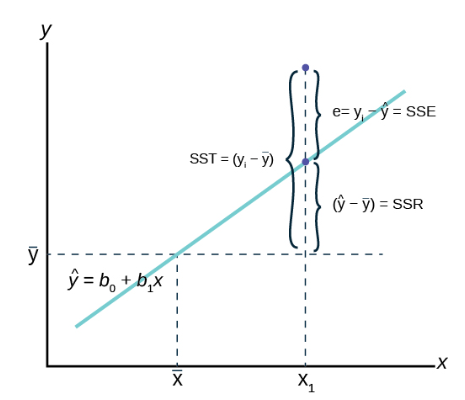
Figure 25 shows the estimated regression line and a single observation,  . Regression analysis tries to explain the variation of the data about the mean value of the dependent variable, y. The question is, why do the observations of y vary from the average level of y? The value of y at observation varies from the mean of y by the difference
  .). The sum of these differences squared is SST, the sum of squares total. The actual value of y at deviates from the estimated value, , by the difference between the estimate value and the actual value,
  . We recall that this is the error term, e, and the sum of these errors is SSE, sum of squared errors. The deviation of the predicted value of y, , from the mean value of y is
  and is the SSR, sum of squares regression. It is called “regression” because it is the deviation explained by the regression. (Sometimes the SSR is called SSM for sum of squares mean because it measures the deviation from the mean value of the dependent variable, y, as shown on the graph.).
Because the SST = SSR + SSE we see that the multiple correlation coefficient is the percent of the variance, or deviation in y from its mean value, that is explained by the equation when taken as a whole.  will vary between zero and 1, with zero indicating that none of the variation in y was explained by the equation and a value of 1 indicating that 100% of the variation in y was explained by the equation. For time series studies expect a high and for cross-section data expect low .
While a high is desirable, remember that it is the tests of the hypothesis concerning the existence of a relationship between a set of independent variables and a particular dependent variable that was the motivating factor in using the regression model. It is validating a cause-and-effect relationship developed by some theory that is the true reason that we chose the regression analysis. Increasing the number of independent variables will have the effect of increasing . To account for this effect the proper measure of the coefficient of determination is  , adjusted for degrees of freedom, to keep down mindless addition of independent variables.
There is no statistical test for the and thus little can be said about the model using with our characteristic confidence level. Two models that have the same size of SSE, that is sum of squared errors, may have very different if the competing models have different SST, total sum of squared deviations. The goodness of fit of the two models is the same; they both have the same sum of squares unexplained, errors squared, but because of the larger total sum of squares on one of the models the differs. Again, the real value of regression as a tool is to examine hypotheses developed from a model that predicts certain relationships among the variables. These are tests of hypotheses on the coefficients of the model and not a game of maximizing .
R-Squared or Coefficient of Determination
Data Analysis Tools (Spreadsheets and Basic Programming)
Descriptive Statistics
Using Microsoft Excel’s “Descriptive Statistics” Tool
How to Run Descriptive Statistics in R
Descriptive Statistics in R Part 2
Regression Analysis
How to Use Microsoft Excel for Regression Analysis
Please read this text on how to use Microsoft Excel for regression analysis.
Simple Linear Regression in Excel
Simple Linear Regression, fit and interpretations in R
Relevance to Transportation Engineering Coursework
This section explains the relevance of the regression models for trip generation, mode choice, traffic flow-speed-density relationship, traffic safety, and appropriate sample size for spot speed study to transportation engineering coursework.
Regression Models for Trip Generation
The trip generation step is the first of the four-step process for estimating travel demand for infrastructure planning. It involves estimating the number of trips made to and from each traffic analysis zone (TAZ). Trip generation models are estimated based on land use and trip-making data. They use either linear regression or cross-tabulation of household characteristics. Simple linear regression is described in the section above titled “Compute and Interpret Simple Linear Regression Between Two Variables”, and the tools to conduct the linear regression are discussed in “Data Analysis Tools (Spreadsheets and Basic Programming)”.
Mode Choice
Estimation of Mode Choice is also part of the four-step process for estimating travel demand. It entails estimating the trip makers’ transportation mode (drive alone, walk, take public transit, etc.) choices. The results of this step are the counts of trips categorized by mode. The most popular mode choice model is the discrete choice, multinomial logit model. Hypothesis tests are conducted for the estimated model parameters to assess whether they are “statistically significant.” The section titled “Use Specific Significance Tests Including, Z-Test, T-Test (one and two samples), Chi-Squared Test” of this chapter provides extensive information on hypothesis testing.
Traffic Flow-Speed-Density Relationship
Greenshield’s model is used to represent the traffic flow-speed-density relationship. Traffic speed and traffic density (number of vehicles per unit mile) are collected to estimate a linear regression model for speed as a function of density. “Compute and Interpret Simple Linear Regression Between Two Variables” above provides information on simple linear regression. “Data Analysis Tools (Spreadsheets and Basic Programming)” provides guidance for implementing the linear regression technique using tools available in Microsoft Excel and the programing language R.
Traffic Safety
Statistical analyses of traffic collisions are used to estimate traffic safety in roadway locations. A variety of regression models, most of which are beyond the scope of this book, are implemented to investigate the association between crashes and characteristics of the roadway locations. Hypothesis tests are conducted for the estimated model parameters to assess whether they are “statistically significant.” “Find Confidence Intervals for Parameter Estimates” above describes the confidence intervals of the parameters, and “Use Specific Significance Tests Including, Z-Test, T-Test (one and two samples), Chi-Squared Test” discusses the different types of hypothesis tests. Programing language R includes statistical analysis toolkits or packages that may be used to estimate the regression models for crash data.
Appropriate Sample Size for Spot Speed Study
Spot speed studies during relatively congestion-free durations are conducted to estimate mean speed, modal speed, pace, standard deviation, and different percentile of speeds at a roadway location. An adequate number of data points (i.e., the number of vehicle speeds recorded) are required to ensure reliable results within an acceptable margin of error. “Estimate the Required Sample Size for Testing” in this chapter discusses the approach to assessing the adequacy of sample size.
Key Takeaways
- Estimating the total number of trips made to and from each traffic analysis zone (TAZ)is typically the first step in the four-step travel demand modeling process. Simple linear regression models and the tools (such as MS Excel and R) to estimate these models are used this step of the travel demand modeling process. The independent variables for these models are the total number of trips with demographic and employment data for the zones as independent variables.
- Hypothesis testing is used to determine the statistical significance of coefficients estimated for the discrete choice multinomial models. Such models are used for the mode choice step of the travel demand modeling process.
- Linear regression models are also used to estimate the relationship between speed and density on uninterrupted flow facilities such as freeway segments.
- Regression models are also implemented to investigate the association between crashes and characteristics of the roadway locations. Tools described in the chapter for linear regression may also be used for estimating these models, including negative binomial regression models.
- Statistical analysis is also used to ensure that an adequate number of data points (i.e., the number of vehicle speeds recorded) are used to obtain estimates of the mean, median, and 85th percentile of speed within an acceptable margin of error in a spot speed study.
Glossary – Key Terms
where SSR is the “sum of squares regressions” and SST is the “sum of squares total.” The appropriate coefficient of determination to be reported should always be adjusted for degrees of freedom firstAnalysis of Variance[1] – also referred to as ANOVA, is a method of testing whether or not the means of three or more populations are equal. The method is applicable if: (1) all populations of interest are normally distributed (2) the populations have equal standard deviations (3) samples (not necessarily of the same size) are randomly and independently selected from each population (4) there is one independent variable and one dependent variable. The test statistic for analysis of variance is the F-ratio
Average[1] – a number that describes the central tendency of the data; there are a number of specialized averages, including the arithmetic mean, weighted mean, median, mode, and geometric mean.
B is the Symbol for Slope[1] – the word coefficient will be used regularly for the slope, because it is a number that will always be next to the letter “x.” It will be written a 𝑏1 when a sample is used, and 𝛽1 will be used with a population or when writing the theoretical linear model.
Binomial Distribution[1] – a discrete random variable which arises from Bernoulli trials; there are a fixed number, n, of independent trials. “Independent” means that the result of any trial (for example, trial 1) does not affect the results of the following trials, and all trials are conducted under the same conditions. Under these circumstances the binomial random variable X is defined as the number of successes in n trials. The notation is: 𝑋~𝐵(𝑛,𝑝). The mean is 𝜇=𝑛𝑝 and the standard deviation is . The probability of exactly x successes in n trials is 
Bivariate[1] – two variables are present in the model where one is the “cause” or independent variable and the other is the “effect” of dependent variable.
Central Limit Theorem[1] – given a random variable with known mean 𝜇 and known standard deviation, 𝜎, we are sampling with size n, and we are interested in two new random variables: the sample mean, . If the size (n) of the sample is sufficiently large, then  . If the size (n) of the sample is sufficiently large, then the distribution of the sample means will approximate a normal distributions regardless of the shape of the population. The mean of the sample means will equal the population mean. The standard deviation of the distribution of the sample means, , is called the standard error of the mean.
Cohen’s d [1] – a measure of effect size based on the differences between two means. If d is between 0 and 0.2 then the effect is small. If d approaches is 0.5, then the effect is medium, and if d approaches 0.8, then it is a large effect.
Confidence Interval (CI)[1] – an interval estimate for an unknown population parameter. This depends on: (1) the desired confidence level (2) information that is known about the distribution (for example, known standard deviation) (3) the sample and its size
Confidence Level (CL)[1] – the percent expression for the probability that the confidence interval contains the true population parameter; for example, if the CL = 90%, then in 90 out of 100 samples the interval estimate will enclose the true population parameter.
Contingency Table[1] – a table that displays sample values for two different factors that may be dependent or contingent on one another; it facilitates determining conditional probabilities.
Critical Value[1] – The t or Z value set by the researcher that measures the probability of a Type I error, 𝛼
Degrees of Freedom (df)[1] – the number of objects in a sample that are free to vary
Error Bound for a Population Mean (EBM)[1] – the margin of error; depends on the confidence level, sample size, and known or estimated population standard deviation.
Error Bound for a Population Proportion (EBP)[1] – the margin of error; depends on the confidence level, the sample size, and the estimated (from the sample) proportion of successes.
Goodness-of-Fit[1] – a hypothesis test that compares expected and observed values in order to look for significant differences within one non-parametric variable. The degrees of freedom used equals the (number of categories – 1).
Hypothesis[1] – a statement about the value of a population parameter, in case of two hypotheses, the statement assumed to be true is called the null hypothesis (notation 𝐻0) and the contradictory statement is called the alternative hypothesis (notation 𝐻𝑎)
Hypothesis Testing[1] – Based on sample evidence, a procedure for determining whether the hypothesis stated is a reasonable statement and should not be rejected, or is unreasonable and should be rejected.
Independent Groups[1] – two samples that are selected from two populations, and the values from one population are not related in any way to the values from the other population.
Inferential Statistics[1] – also called statistical inference or inductive statistics; this facet of statistics deals with estimating a population parameter based on a sample statistic. For example, if four out of the 100 calculators sampled are defective we might infer that four percent of the production is defective.
Linear[1] – a model that takes data and regresses it into a straight line equation.
Matched Pairs[1] – two samples that are dependent. Differences between a before and after scenario are tested by testing one population mean of differences.
Mean[1] – a number that measures the central tendency; a common name for mean is “average.” The term “mean” is a shortened form of “arithmetic mean.” By definition, the mean for a sample (denoted by  , and the mean for a population (denoted by 𝜇) is
Multivariate[1] – a system or model where more than one independent variable is being used to predict an outcome. There can only ever be one dependent variable, but there is no limit to the number of independent variables.
Normal Distribution[1] – a continuous random variable with pdf  , where 𝜇 is the mean of the distribution and 𝜎 is the standard deviation; notation: 𝑋~𝑁(𝜇,𝜎). If 𝜇=0 and 𝜎=1, the random variable, Z, is called the standard normal distribution.
Normal Distribution[1] – a continuous random variable with pdf  , where 𝜇 is the mean of the distribution and 𝜎 is the standard deviation, notation:
One-Way ANOVA[1] – a method of testing whether or not the means of three or more populations are equal; the method is applicable if: (1) all populations of interest are normally distributed (2) the populations have equal standard deviations (3) samples (not necessarily of the same size) are randomly and independently selected from each population. The test statistic for analysis of variance is the F-ratio
Parameter[1] – a numerical characteristic of a population
Point Estimate[1] – a single number computed from a sample and used to estimate a population parameter
Pooled Variance[1] – a weighted average of two variances that can then be used when calculating standard error.
R – Correlation Coefficient[1] – A number between −1 and 1 that represents the strength and direction of the relationship between “X” and “Y.” The value for “r” will equal 1 or −1 only if all the plotted points form a perfectly straight line.
Residual or “Error”[1] – the value calculated from subtracting . The absolute value of a residual measures the vertical distance between the actual value of y and the estimated value of y that appears on the best-fit line.
Sampling Distribution[1] – Given simple random samples of size n from a given population with a measured characteristic such as mean, proportion, or standard deviation for each sample, the probability distribution of all the measured characteristics is called a sampling distribution.
Standard Deviation[1] – a number that is equal to the square root of the variance and measures how far data values are from their mean; notation: s for sample standard deviation and 𝜎 for population standard deviation
Standard Error of the Mean[1] – the standard deviation of the distribution of the sample means, or
Standard Error of the Proportion[1] – the standard deviation of the sampling distribution of proportions
Student’s t-Distribution[1] – investigated and reported by William S. Gossett in 1908 and published under the pseudonym Student; the major characteristics of this random variable are: (1) it is continuous and assumes any real values (2) the pdf is symmetrical about its mean of zero (3) it approaches the standard normal distribution as n gets larger (4) there is a “family” of t-distributions: each representative of the family is completely defined by the number of degrees of freedom, which depends upon the application for which the t is being used.
Sum of Squared Errors (SSE)[1] – the calculated value from adding up all the squared residual terms. The hope is that this value is very small when creating a model.
Test for Homogeneity[1] – a test used to draw a conclusion about whether two populations have the same distribution. The degrees of freedom used equals the (number of columns – 1).
Test of Independence[1] – a hypothesis test that compares expected and observed values for contingency tables in order to test for independence between two variables. The degrees of freedom used equals the (number of columns – 1) multiplied by the (number of rows – 1).
Test Statistic[1] – the formula that counts the number of standard deviations on the relevant distribution that estimated parameter is away from the hypothesized value.
Type I Error[1] – the decision is to reject the null hypothesis when, in fact, the null hypothesis is true.
Type II Error[1] – the decision is not to reject the null hypothesis when, in fact, the null hypothesis is false.
Variance[1] – mean of the squared deviations from the mean; the square of the standard deviation. For a set of data, a deviation can be represented as  where x is a value of the data and is the sample mean. The sample variance is equal to the sum of the squares of the deviations divided by the difference of the sample size and one.
X – the Independent Variable[1] – This will sometimes be referred to as the “predictor” variable, because these values were measured in order to determine what possible outcomes could be predicted.
Y – the Dependent Variable[1] – also, using the letter “y” represents actual values while represents predicted or estimated values. Predicted values will come from plugging in observed “x” values into a linear model
[1] “Introductory Business Statistics” by Alexander Holmes, Barbara Illowsky, and Susan Dean on OpenStax. Access for free at https://openstax.org/books/introductory-business-statistics/pages/1-introduction
Media Attributions
Videos
- Video 1: Central Limit Theorem by Khan Academy is licensed by Creative Commons NonCommercial-ShareAlike 3.0 United States (CC BY-NC-SA 3.0 US)
- Video 2: Sampling Distribution of the Sample Mean by Khan Academy is licensed by Creative Commons NonCommercial-ShareAlike 3.0 United States (CC BY-NC-SA 3.0 US)
- Video 3: Sampling Distribution of the Sample Mean (Part 2) by Khan Academy is licensed by Creative Commons NonCommercial-ShareAlike 3.0 United States (CC BY-NC-SA 3.0 US)
- Video 4: Sampling Distributions: Sampling Distribution of the Mean by Khan Academy is licensed by Creative Commons NonCommercial-ShareAlike 3.0 United States (CC BY-NC-SA 3.0 US)
- Video 5: Confidence Intervals & Estimation: Point Estimates Explained by Linda Williams is licensed by Creative Commons 3.0 Unported (CC BY 3.0)
- Video 6: Confidence Interval for Mean: 1 Sample Z Test (Using Formula) by Linda Williams is licensed by Creative Commons 3.0 Unported (CC BY 3.0)
- Video 7: Confidence Intervals: Using the t Distribution by Linda Williams is licensed by Creative Commons 3.0 Unported (CC BY 3.0)
- Video 8: How to Construct a Confidence Interval for Population Proportion by Simple Science and Maths is licensed by Creative Commons 3.0 Unported (CC BY 3.0)
- Video 9: Estimation and Confidence Intervals: Calculate Sample Size by Linda Williams is licensed by Creative Commons 3.0 Unported (CC BY 3.0)
- Video 10: Calculating Sample size to Predict a Population Proportion by Matthew Simmons is licensed by Creative Commons 3.0 Unported (CC BY 3.0)
- Video 11: Hypothesis Testing: The Fundamentals by Linda Williams is licensed by Creative Commons 3.0 Unported (CC BY 3.0)
- Video 12: Hypothesis Testing: Setting up the Null and Alternative Hypothesis Statements by Linda Williams is licensed by Creative Commons 3.0 Unported (CC BY 3.0)
- Video 13: Hypothesis Testing: Type I and Type II Errors by Linda Williams is licensed by Creative Commons 3.0 Unported (CC BY 3.0)
- Video 14: Hypothesis testing: Finding Critical Values by Linda Williams is licensed by Creative Commons 3.0 Unported (CC BY 3.0)
- Video 15: Normal Distribution: Finding Critical Values of Z by Linda Williams is licensed by Creative Commons 3.0 Unported (CC BY 3.0)
- Video 16: What is a “P-Value?” by Linda Williams is licensed by Creative Commons 3.0 Unported (CC BY 3.0)
- Video 17: Hypothesis Testing: One Sample Z Test of the Mean (Critical Value Approach) by Linda Williams is licensed by Creative Commons 3.0 Unported (CC BY 3.0)
- Video 18: Hypothesis Testing: t Test for the Mean (Critical Value Approach)by Linda Williams is licensed by Creative Commons 3.0 Unported (CC BY 3.0)
- Video 19: Hypothesis Testing: 1 Sample Z Test of the Mean (Confidence Interval Approach) by Linda Williams is licensed by Creative Commons 3.0 Unported (CC BY 3.0)
- Video 20: Hypothesis Testing: 1 Sample Z Test for Mean (P-Value Approach) by Linda Williams is licensed by Creative Commons 3.0 Unported (CC BY 3.0)
- Video 21: Hypothesis Testing: 1 Proportion using the Critical Value Approach by Linda Williams is licensed by Creative Commons 3.0 Unported (CC BY 3.0)
- Video 22: Hypothesis Testing – Two Population Means by Peter Dalley is licensed by Creative Commons 3.0 Unported (CC BY 3.0)
- Video 23: Two Population Means, One Tail Test, unknown by Peter Dalley is licensed by Creative Commons 3.0 Unported (CC BY 3.0)
- Video 24: Two Population Means, Two Tail Test, unknown by Peter Dalley is licensed by Creative Commons 3.0 Unported (CC BY 3.0)
- Video 25: Effect Size for a Significant Difference of Two Sample Means by Dana Lee Ling is licensed by Creative Commons 3.0 Unported (CC BY 3.0)
- Video 26: Two Population Means, One Tail Test, Known by Peter Dalley is licensed by Creative Commons 3.0 Unported (CC BY 3.0)
- Video 27: Two Population Means, Two Tail Test, Known by Peter Dalley is licensed by Creative Commons 3.0 Unported (CC BY 3.0)
- Video 28: Two Population Means, One Tail Test, Matched Sample by Peter Dalley is licensed by Creative Commons 3.0 Unported (CC BY 3.0)
- Video 29: Two Population Means, One Tail test, Matched Sample by Peter Dalley is licensed by Creative Commons 3.0 Unported (CC BY 3.0)
- Video 30: Matched Sample, Two Tail Test by Peter Dalley is licensed by Creative Commons 3.0 Unported (CC BY 3.0)
- Video 31: Two Population Proportions, One Tail Test by Peter Dalley is licensed by Creative Commons 3.0 Unported (CC BY 3.0)
- Video 32: Two Population Proportion, Two Tail Test by Peter Dalley is licensed by Creative Commons 3.0 Unported (CC BY 3.0)
- Video 33: Single Population Variances, One-Tail Test by Peter Dalley is licensed by Creative Commons 3.0 Unported (CC BY 3.0)
- Video 34: Chi-Square Statistic for Hypothesis Testing by Khan Academy is licensed by Creative Commons NonCommercial-ShareAlike 3.0 United States (CC BY-NC-SA 3.0 US)
- Video 35: Chi-Square Goodness-of-Fit Example by Khan Academy is licensed by Creative Commons NonCommercial-ShareAlike 3.0 United States (CC BY-NC-SA 3.0 US)
- Video 36: Simple Explanation of Chi-Squared by J David Eisenberg is licensed by Creative Commons 3.0 Unported (CC BY 3.0)
- Video 37: Chi-Square Tet for Association (independence)by Khan Academy is licensed by Creative Commons NonCommercial-ShareAlike 3.0 United States (CC BY-NC-SA 3.0 US)
- Video 38: Introduction to the Chi-Square Test for Homogeneity by Khan Academy is licensed by Creative Commons NonCommercial-ShareAlike 3.0 United States (CC BY-NC-SA 3.0 US)
- Video 39: Hypothesis Test Two Population Variances by Peter Dalley is licensed by Creative Commons 3.0 Unported (CC BY 3.0)
- Video 40: ANOVA by J David Eisenberg is licensed by Creative Commons 3.0 Unported (CC BY 3.0)
- Video 41: Calculating SST (total sum of squares) by Khan Academy is licensed by Creative Commons NonCommercial-ShareAlike 3.0 United States (CC BY-NC-SA 3.0 US)
- Video 42: Calculating by Khan Academy is licensed by Creative Commons NonCommercial-ShareAlike 3.0 United States (CC BY-NC-SA 3.0 US)
- Video 43: Hypothesis Test with F-Statistic by Khan Academy is licensed by Creative Commons NonCommercial-ShareAlike 3.0 United States (CC BY-NC-SA 3.0 US)
- Video 44: Bivariate Relationship Linearity, Strength, and Direction by Khan Academy is licensed by Creative Commons NonCommercial-ShareAlike 3.0 United States (CC BY-NC-SA 3.0 US)
- Video 45: Calculating Correlation Coefficient r by Khan Academy is licensed by Creative Commons NonCommercial-ShareAlike 3.0 United States (CC BY-NC-SA 3.0 US)
- Video 46: Example: Correlation Coefficient Intuition by Khan Academy is licensed by Creative Commons NonCommercial-ShareAlike 3.0 United States (CC BY-NC-SA 3.0 US)
- Video 47: Introduction to Residuals and Least-Squares Regression by Khan Academy is licensed by Creative Commons NonCommercial-ShareAlike 3.0 United States (CC BY-NC-SA 3.0 US)
- Video 48: Calculating Residual Example by Khan Academy is licensed by Creative Commons NonCommercial-ShareAlike 3.0 United States (CC BY-NC-SA 3.0 US)
- Video 49: Residual Plots by Khan Academy is licensed by Creative Commons NonCommercial-ShareAlike 3.0 United States (CC BY-NC-SA 3.0 US)
- Video 50: Calculating the Equation of a Regression Line by Khan Academy is licensed by Creative Commons NonCommercial-ShareAlike 3.0 United States (CC BY-NC-SA 3.0 US)
- Video 51: Interpreting Slope of Regression Line by Khan Academy is licensed by Creative Commons NonCommercial-ShareAlike 3.0 United States (CC BY-NC-SA 3.0 US)
- Video 52: Interpreting y-intercept in Regression Model by Khan Academy is licensed by Creative Commons NonCommercial-ShareAlike 3.0 United States (CC BY-NC-SA 3.0 US)
- Video 53: Using Least Squares Regression Output by Khan Academy is licensed by Creative Commons NonCommercial-ShareAlike 3.0 United States (CC BY-NC-SA 3.0 US)
- Video 54: R-Squared or Coefficient of Determination by Khan Academy is licensed by Creative Commons NonCommercial-ShareAlike 3.0 United States (CC BY-NC-SA 3.0 US)
- Video 55: Using Microsoft Excel’s “Descriptive Statistics” Tool by Linda Weiser Friedman is licensed by Creative Commons 3.0 Unported (CC BY 3.0)
- Video 56: How to Run Descriptive Statistics in R by Learning Puree is licensed by Creative Commons 4.0 International (CC BY 4.0)
- Video 57: Descriptive Statistics in R Part 2 by Learning Puree is licensed by Creative Commons 4.0 International (CC BY 4.0)
- Video 58: Simple Linear Regression in Excel by Ramya Rachel is licensed by Creative Commons 3.0 Unported (CC BY 3.0)
- Video 59: Simple Linear Regression, fit and interpretations in Ris licensed by Creative Commons 3.0 Unported (CC BY 3.0)
Figures
- Figure 1: “Introductory Business Statistics” by Alexander Holmes, Barbara Illowsky, and Susan Dean is licensed by Creative Commons 4.0 International (CC BY 4.0)
- Figure 2: “Introductory Business Statistics” by Alexander Holmes, Barbara Illowsky, and Susan Dean is licensed by Creative Commons 4.0 International (CC BY 4.0)
- Figure 3: “Introductory Business Statistics” by Alexander Holmes, Barbara Illowsky, and Susan Dean is licensed by Creative Commons 4.0 International (CC BY 4.0)
- Figure 4: “Introductory Business Statistics” by Alexander Holmes, Barbara Illowsky, and Susan Dean is licensed by Creative Commons 4.0 International (CC BY 4.0)
- Figure 5: “Introductory Business Statistics” by Alexander Holmes, Barbara Illowsky, and Susan Dean is licensed by Creative Commons 4.0 International (CC BY 4.0)
- Figure 6: “Introductory Business Statistics” by Alexander Holmes, Barbara Illowsky, and Susan Dean is licensed by Creative Commons 4.0 International (CC BY 4.0)
- Figure 7: “Introductory Business Statistics” by Alexander Holmes, Barbara Illowsky, and Susan Dean is licensed by Creative Commons 4.0 International (CC BY 4.0)
- Figure 8: “Introductory Business Statistics” by Alexander Holmes, Barbara Illowsky, and Susan Dean is licensed by Creative Commons 4.0 International (CC BY 4.0)
- Figure 9: “Introductory Business Statistics” by Alexander Holmes, Barbara Illowsky, and Susan Dean is licensed by Creative Commons 4.0 International (CC BY 4.0)
- Figure 10: “Introductory Business Statistics” by Alexander Holmes, Barbara Illowsky, and Susan Dean is licensed by Creative Commons 4.0 International (CC BY 4.0)
- Figure 11: “Introductory Business Statistics” by Alexander Holmes, Barbara Illowsky, and Susan Dean is licensed by Creative Commons 4.0 International (CC BY 4.0)
- Figure 12: “Introductory Business Statistics” by Alexander Holmes, Barbara Illowsky, and Susan Dean is licensed by Creative Commons 4.0 International (CC BY 4.0)
- Figure 13: “Introductory Business Statistics” by Alexander Holmes, Barbara Illowsky, and Susan Dean is licensed by Creative Commons 4.0 International (CC BY 4.0)
- Figure 14: by Alexander Holmes, Barbara Illowsky, and Susan Dean is licensed by Creative Commons 4.0 International (CC BY 4.0)
- Figure 15 by Alexander Holmes, Barbara Illowsky, and Susan Dean is licensed by Creative Commons 4.0 International (CC BY 4.0)
- Figure 16 by Alexander Holmes, Barbara Illowsky, and Susan Dean is licensed by Creative Commons 4.0 International (CC BY 4.0)
- Figure 17 by Alexander Holmes, Barbara Illowsky, and Susan Dean is licensed by Creative Commons 4.0 International (CC BY 4.0)
- Figure 18 by Alexander Holmes, Barbara Illowsky, and Susan Dean is licensed by Creative Commons 4.0 International (CC BY 4.0)
- Figure 19 by Alexander Holmes, Barbara Illowsky, and Susan Dean is licensed by Creative Commons 4.0 International (CC BY 4.0)
- Figure 20 by Alexander Holmes, Barbara Illowsky, and Susan Dean is licensed by Creative Commons 4.0 International (CC BY 4.0)
- Figure 21 by Alexander Holmes, Barbara Illowsky, and Susan Dean is licensed by Creative Commons 4.0 International (CC BY 4.0)
- Figure 22 by Alexander Holmes, Barbara Illowsky, and Susan Dean is licensed by Creative Commons 4.0 International (CC BY 4.0)
- Figure 23 by Alexander Holmes, Barbara Illowsky, and Susan Dean is licensed by Creative Commons 4.0 International (CC BY 4.0)
- Figure 24 by Alexander Holmes, Barbara Illowsky, and Susan Dean is licensed by Creative Commons 4.0 International (CC BY 4.0)
- Figure 25 by Alexander Holmes, Barbara Illowsky, and Susan Dean is licensed by Creative Commons 4.0 International (CC BY 4.0)
References
Note: All Khan Academy content is available for free at (www.khanacademy.org).
- “Unit: Sampling Distributions” by Khan Academy is licensed by Creative Commons NonCommercial-ShareAlike 3.0 United States (CC BY-NC-SA 3.0 US)
- “Unit: Inference for Categorical Data: Chi-Square” by Khan Academy is licensed by Creative Commons NonCommercial-ShareAlike 3.0 United States (CC BY-NC-SA 3.0 US)
- “Unit: Analysis of Variance (ANOVA)” by Khan Academy is licensed by Creative Commons NonCommercial-ShareAlike 3.0 United States (CC BY-NC-SA 3.0 US)
- “Unit: Exploring Two-Variable Quantitative Data” by Khan Academy is licensed by Creative Commons NonCommercial-ShareAlike 3.0 United States (CC BY-NC-SA 3.0 US)
- “Statistics” by Barbara Illosky and Susan Dean is licensed by Creative Commons 4.0 International (CC BY 4.0)
- “Introduction to Probability and Statistics” by Jeremy Orloff and Jonathan Bloom is licensed by Creative Commons NonCommercial-ShareAlike 4.0 International (CC BY-NC-SA 4.0)
- Farid, A. (2022). Transportation Planning 1. Personal Collection of Ahmed Farid, California Polytechnic State University, San Luis Obispo, CA.
- Farid, A. (2022). Transportation Planning 2. Personal Collection of Ahmed Farid, California Polytechnic State University, San Luis Obispo, CA.
- Farid, A. (2022). Fundamentals of Traffic Flow Theory. Personal Collection of Ahmed Farid, California Polytechnic State University, San Luis Obispo, CA.
- Washington, S., Karlaftis, M., Mannering, F., and Anastasopoulos, P. (2020). Statistical and Econometric Methods for Transportation Data Analysis 3rd Edition. Chemical Rubber Company (CRC) Press, Taylor and Francis Group, Boca Raton, FL.
- Farid, A. (2022). Spot Speed Study. Personal Collection of Ahmed Farid, California Polytechnic State University, San Luis Obispo, CA.
Given simple random samples of size n from a given population with a measured characteristic such as mean, proportion, or standard deviation for each sample, the probability distribution of all the measured characteristics is called a sampling distribution.
a mean score is an average score. It is the sum of individual scores divided by the number of individuals.
a numerical characteristic of a population
The standard deviation is a numerical value used to indicate how widely individuals in a group vary. If individual observations vary greatly from the group mean, the standard deviation is big; and vice versa. It is important to distinguish between the standard deviation of a population and the standard deviation of a sample. They have different notation, and they are computed differently. The standard deviation of a population is denoted by 𝜎 and the standard deviation of a sample, by 𝑠
a single number computed from a sample and used to estimate a population parameter
also called statistical inference or inductive statistics; this facet of statistics deals with estimating a population parameter based on a sample statistic. For example, if four out of the 100 calculators sampled are defective we might infer that four percent of the production is defective.
a number that describes the central tendency of the data; there are a number of specialized averages, including the arithmetic mean, weighted mean, median, mode, and geometric mean.
an interval estimate for an unknown population parameter. This depends on: (1) the desired confidence level (2) information that is known about the distribution (for example, known standard deviation) (3) the sample and its size
the margin of error; depends on the confidence level, sample size, and known or estimated population standard deviation.
the percent expression for the probability that the confidence interval contains the true population parameter; for example, if the CL = 90%, then in 90 out of 100 samples the interval estimate will enclose the true population parameter.
investigated and reported by William S. Gossett in 1908 and published under the pseudonym Student; the major characteristics of this random variable are: (1) it is continuous and assumes any real values (2) the pdf is symmetrical about its mean of zero (3) it approaches the standard normal distribution as n gets larger (4) there is a “family” of t-distributions: each representative of the family is completely defined by the number of degrees of freedom, which depends upon the application for which the t is being used.
the number of objects in a sample that are free to vary
a statement about the value of a population parameter, in case of two hypotheses, the statement assumed to be true is called the null hypothesis (notation and the contradictory statement is called the alternative hypothesis
Based on sample evidence, a procedure for determining whether the hypothesis stated is a reasonable statement and should not be rejected, or is unreasonable and should be rejected.
The decision is to reject the null hypothesis when, in fact, the null hypothesis is true.
The decision is not to reject the null hypothesis when, in fact, the null hypothesis is false.
The formula that counts the number of standard deviations on the relevant distribution that estimated parameter is away from the hypothesized value.
The t or Z value set by the researcher that measures the probability of a Type I error, 𝛼
a discrete random variable which arises from Bernoulli trials; there are a fixed number, n, of independent trials. “Independent” means that the result of any trial (for example, trial 1) does not affect the results of the following trials, and all trials are conducted under the same conditions.
two samples that are dependent. Differences between a before and after scenario are tested by testing one population mean of differences.
two samples that are selected from two populations, and the values from one population are not related in any way to the values from the other population.
a measure of effect size based on the differences between two means. If d is between 0 and 0.2 then the effect is small. If d approaches is 0.5, then the effect is medium, and if d approaches 0.8, then it is a large effect.
the variance is a numerical value used to indicate how widely individuals in a group vary. If individual observations vary greatly from the group mean, the variance is big; and vice versa. It is important to distinguish between the variance of a population and the variance of a sample. They have different notation, and they are computed differently.
a hypothesis test that compares expected and observed values in order to look for significant differences within one non-parametric variable. The degrees of freedom used equals the (number of categories – 1).
a table that displays sample values for two different factors that may be dependent or contingent on one another; it facilitates determining conditional probabilities.
a hypothesis test that compares expected and observed values for contingency tables in order to test for independence between two variables. The degrees of freedom used equals the (number of columns – 1) multiplied by the (number of rows – 1).
a test used to draw a conclusion about whether two populations have the same distribution. The degrees of freedom used equals the (number of columns – 1).
also referred to as ANOVA, is a method of testing whether or not the means of three or more populations are equal. The method is applicable if: (1) all populations of interest are normally distributed (2) the populations have equal standard deviations (3) samples (not necessarily of the same size) are randomly and independently selected from each population (4) there is one independent variable and one dependent variable. The test statistic for analysis of variance is the F-ratio
a method of testing whether or not the means of three or more populations are equal; the method is applicable if: (1) all populations of interest are normally distributed (2) the populations have equal standard deviations (3) samples (not necessarily of the same size) are randomly and independently selected from each population. The test statistic for analysis of variance is the F-ratio
a weighted average of two variances that can then be used when calculating standard error.
two variables are present in the model where one is the “cause” or independent variable and the other is the “effect” of dependent variable.
a system or model where more than one independent variable is being used to predict an outcome. There can only ever be one dependent variable, but there is no limit to the number of independent variables.
A number between −1 and 1 that represents the strength and direction of the relationship between “X” and “Y.” The value for “r” will equal 1 or −1 only if all the plotted points form a perfectly straight line.
a model that takes data and regresses it into a straight line equation.
This will sometimes be referred to as the “predictor” variable, because these values were measured in order to determine what possible outcomes could be predicted.
also, using the letter “y” represents actual values while 𝑦ˆ represents predicted or estimated values. Predicted values will come from plugging in observed “x” values into a linear model
The absolute value of a residual measures the vertical distance between the actual value of y and the estimated value of y that appears on the best-fit line.
the calculated value from adding up all the squared residual terms. The hope is that this value is very small when creating a model.
this is a number between 0 and 1 that represents the percentage variation of the dependent variable that can be explained by the variation in the independent variable.
the standard deviation of the distribution of the sample means
